Sequencing Quality Control

Overview

Teaching: 180 min
Exercises: 0 min

Objectives

• Understand the value of sequencing quality control

• Discuss how low quality reads affect genomic analysis

• Perform quality check on long-read data by creating plots

• Interpret quality check results

• Perform quality control on reads

Every step of a metagenomics/viromics analysis pipeline needs quality control and sanity checks.

• What data am I working with?
• What is the quality of the data or analysis?
• Are my results what I expected them to be? Why?/Why not?

Here, we will assess the quality of DNA sequencing.

Sequencing quality control can include:

• Removing barcodes (i.e. oligonucleotides that were artificially added to identify sequences from a particular sample)
• Removing sequencing adapters (i.e. oligonucleotides that were artificially added to facilitate the sequencing process)
• Removing low-quality nucleotides (sequencing quality often drops towards the end of the reads)
• Filtering out reads based on quality scores (some reads are derived from faulty clusters or pores, and are best ignored)

To prepare your data, we used Nanopore basecaller Dorado to do the basecalling and demultiplexing. This step also trims any adapters, primers and barcodes from the reads.

Exercise

Discuss with your classmates and TAs:

1. Why do we need quality control?
2. What are some metrics for assessing sequencing quality?
3. What are the potential impacts of not performing quality control on your reads?

Assessing Sequencing Quality

We will use NanoPlot to assess the quality of our reads. NanoPlot is designed for long reads and uses information in the sequence files to evaluate the quality of our reads.

Exercise

4. Run NanoPlot on your reads
   • Assess the sequencing quality for each sample using default parameters
   • Use fastq files and summary.txt located ./data/sequences/ to generate diff types of quality plots (see the NanoPlot github)
   • Play around with the parameters such as colours and types of plots to generate

# to run nanoplot - you will need to source and activate the following conda environment:
source /vast/groups/VEO/tools/anaconda3/etc/profile.d/conda.sh && conda activate nanoplot_v1.41.3

NanoPlot -t ? --plots ? --color ? --fastq barcode1.fastq.gz -o output_dir/barcode1

Resources

Information about Nanopore sequencing quality and Phred scores

An example sbatch script

How to write a for-loop to loop through your files

sbatch script for NanoPlot

#!/bin/bash
#SBATCH --tasks=1
#SBATCH --cpus-per-task=10
#SBATCH --partition=short,standard,interactive
#SBATCH --mem=1G
#SBATCH --time=2:00:00
#SBATCH --job-name=sequencing_QC
#SBATCH --output=1.1_QC/10_nanoplot/nanoplot.slurm.out.%j
#SBATCH --error=1.1_QC/10_nanoplot/nanoplot.slurm.err.%j

# First, we check the quality of the reads using nanoplot
# activate the conda environment containing nanoplot

source /vast/groups/VEO/tools/anaconda3/etc/profile.d/conda.sh && conda activate nanoplot_v1.41.3

datadir="./data/sequences"
outdir="./1.1_QC/10_nanoplot"

# Run nanoplot on 3 fastq files in a for loop
# -t : threads (cpus)
# --plots : types of plots to produce, see gallery: https://gigabaseorgigabyte.wordpress.com/2017/06/01/example-gallery-of-nanoplot/ 
# --N50 : draw the N50 vertical line on the plots
# --color : color for the plots
# -o : output directory
# to see other options for colors and prefilters, run : NanoPlot -h

for fn in $datadir/*.fastq.gz
do
base_f=$(basename $fn .fastq.gz)        # select just the first part of the name
NanoPlot -t 10 --plots dot --N50 --color slateblue --fastq $fn -o $outdir/${base_f}/
done

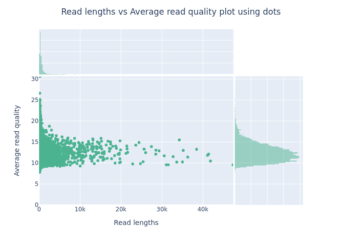
This is an example of a plot you might get from NanoPlot. It is important to look at such a plot to estimate how much data will be lost when you filter by read quality or length.

• The top plot shows frequency of read lengths
• The large main plot shows how the read quality changes by read length
• The right plot shows the frequency of read qualities

Exercise

5. How does the sequencing quality of the 2 samples compare to each other? Specify your answer with metrics from the NanoPlot results.
6. Do we need to remove any reads? Why (not)?
7. What does Q12 mean? How much data will be lost from each sample if we filter at Q12?

Filtering Reads

Many phages naturally have low-complexity regions in their genomes (e.g. ACACACACAC). Nanopore sequencing errors are biased towards low-complexity regions, either by falsely generating them or by exacerbating them. This can create artefacts in the assembled viral genome sequences. High-quality reads can significantly improve assemblies, particularly for error-prone long reads.

Exercise - filter your reads

7. We will use Chopper to filter our reads based on quality scores and length. Build an sbatch script for chopper based on the following basic usage example. Use a for-loop that processes all your reads files. Use the following filtering criteria:
   • minimum quality 14
   • minimum length 1000 bp
   • maximum length 40000 bp

# activate the conda environment
source /vast/groups/VEO/tools/anaconda3/etc/profile.d/conda.sh && conda activate chopper_v0.5.0

# base usage for filtering with minimum quality 14
gunzip -c reads.fastq.gz | chopper -q 14| gzip > filtered_reads.fastq.gz

# check the help for the other options
chopper -h

Chopper sbatch example

#!/bin/bash
#SBATCH --tasks=1
#SBATCH --cpus-per-task=10
#SBATCH --partition=short,standard
#SBATCH --mem=1G
#SBATCH --time=2:00:00
#SBATCH --job-name=sequencing_QC
#SBATCH --output=1.1_QC/20_chopper/chopper.slurm.out.%j
#SBATCH --error=1.1_QC/20_chopper/chopper.slurm.err.%j

# activate the conda environment containing chopper

source /vast/groups/VEO/tools/anaconda3/etc/profile.d/conda.sh && conda activate chopper_v0.5.0

datadir="./data/sequences"
outdir="1.1_QC/20_chopper"

# gunzip : unzip the reads
# -q : minimum read quality to keep
# -l : minimum read length to keep
# gzip: rezip the filtered reads

for fn in ./data/sequences/*.fastq.gz
do

base_f=$(basename $fn .fastq.gz)        # select just the first part of the name
gunzip -c $fn | chopper -q 14 -l 1000 --maxlength 40000 | gzip > $outdir/${base_f}_filtered_reads.fastq.gz

done

Exercise

8. How many reads do you have left after filtering? What percentage of the original reads were filtered?
9. What is the average quality before and after filtering?
10. Optional: Run Nanoplot again to show the difference in the read statistics

GC Content

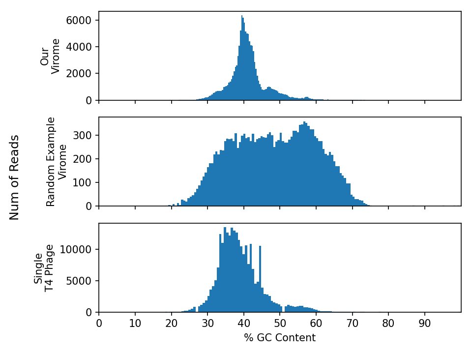
GC Content ((sum of all G’s + C’s) / (sum of all T’s + A’s)) is another interesting metric to evaluate your sequencing data. There’s no “wrong” GC content, rather this measure tells us something about the nucleic acid diversity our metagenomes/viromes. GC content is generally consistent along the length of a genome, as the GC content of sequencing reads from a single genome follows a bell curve. Regions with outlier values often represent non-self regions, for example a horizontally transferred gene, an inserted prophage, or a mobile genetic element. GC content is generally consistent for genomes of similar strains.

Below are three GC plots - viromes from 2 samples + an E. coli phage T4 phage genome. Please use this plot to answer the following questions.

Exercise - GC content plots

Interpret the distributions:

1. Are these histograms what you expected?
2. How would the GC content of a metagenome differ from these viromes?
3. Describe the difference in GC content between our viromes and E. coli phage T4.
4. What interpretations can you make about the samples based on these plots?

Below is the python script used to make these plots for your reference and future use.

python script to make GC_content plots

To install the libraries

source ./py3env/bin/activate
pip install biopython, pandas, numpy, matplotlib

#! usr/bin/python3

# import libraries into your script
from Bio.SeqUtils import gc_fraction
from Bio import SeqIO
import pandas as pd
import numpy as np
import gzip, sys
import matplotlib.pyplot as plt

fastq_dir=sys.argv[1]
T4_path=sys.argv[2]

# read in fastq.gz files 
gc_62={}
with gzip.open(f"{fastq_dir}/full_barcode62_filtered_reads.fastq.gz", 'rt') as f:
   for record in SeqIO.parse(f, "fastq"):
       gc_62[record.id]=gc_fraction(record.seq)*100

print("gc_62... done")

gc_63={}
with gzip.open(f"{fastq_dir}/full_barcode62_filtered_reads.fastq.gz", 'rt') as f:
   for record in SeqIO.parse(f, "fastq"):
       gc_63[record.id]=gc_fraction(record.seq)*100
print("gc_63... done")

gc_64={}
with gzip.open(f"{fastq_dir}/full_barcode62_filtered_reads.fastq.gz", 'rt') as f:
   for record in SeqIO.parse(f, "fastq"):
       gc_64[record.id]=gc_fraction(record.seq)*100
print("gc_64... done")

gc_T4={}
with gzip.open(T4_path, 'rt') as f:
   for record in SeqIO.parse(f, "fastq"):
       gc_T4[record.id]=gc_fraction(record.seq)*100
       #print(gc_fraction(record.seq)*100)
print("gc_T4... done")

# convert to a pandas dataframe
# For your samples
df_62 = pd.DataFrame([gc_62])
df_62 = df_62.T
df_63 = pd.DataFrame([gc_63])
df_63 = df_63.T
df_64 = pd.DataFrame([gc_64])
df_64 = df_64.T

# For T4 phage
df_T4 = pd.DataFrame([gc_T4])
df_T4 = df_T4.T

# make a plotting function
def make_plot(axs):
   # We can set the number of bins with the *bins* keyword argument.
   n_bins = 150

   ax1 = axs[0]
   ax1.hist(df_62, bins=n_bins)
   ax1.set_title('% GC content')
   ax1.set_ylabel('Barcode 62')
   ax1.set_xlim(0, 100)
   ax1.set_xticks(np.arange(0, 100, step=10))

   ax2 = axs[1]
   ax2.hist(df_63, bins=n_bins)
   ax2.set_ylabel('Barcode 63')

   ax3 = axs[2]
   ax3.hist(df_64, bins=n_bins)
   ax3.set_ylabel('Barcode 64')

   ax4 = axs[3]
   ax4.hist(df_T4, bins=n_bins)
   ax4.set_ylabel('T4 Phage')

# Plot:
fig, axs = plt.subplots(4,1, sharex=True, tight_layout=True)
make_plot(axs)
plt.show()

# save your plot
fig.savefig('GC_Content.png', dpi=150)

Key Points

• Sequencing quality control is an important first evaluation of our data

• NanoPlot can be used to evaluate read quality of long reads

• Chopper can be used to filter reads based on quality and/or length

• The GC content profile of a metagenome or virome is composed of a mix of bell curves