Introduction
Overview
Teaching: 10 min
Exercises: 0 minQuestions
What is metagenomics
What do we call viral dark matter
Objectives
Understanding what is a metagenomic study
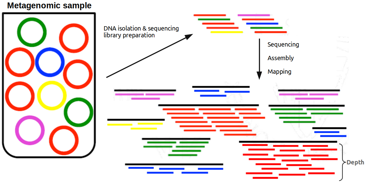
The emergence of Next Generation Sequencing (NGS) has facilitated the development of metagenomics. In metagenomic studies, DNA from all the organisms in a mixed sample is sequenced in a massively parallel way (or RNA in case of metatranscriptomics). The goal of these studies is usually to identify certain microbes in a sample, or to taxonomically or functionally characterize a microbial community. There are different ways to process and analyze metagenomes, such as the targeted amplification and sequencing of the 16S ribosomal RNA gene (amplicon sequencing, used for taxonomic profiling) or shotgun sequencing of the complete genomes (metagenomics, used for taxonomic and functional profiling).
After primary processing including quality control of the sequencing data (which we will not perform in this exercise), the metagenomic sequences are compared to a reference database composed of genome sequences of known organisms. Sequence similarity indicates that the microbes in the sample are genomically related to the organisms in the database. By counting the sequencing reads that are related to certain taxa, or that encode certain functions, we can get an idea of the ecology and functioning of the sampled metagenome.
When the sample is composed mostly of viruses we talk of metaviromics. Viruses are the most abundant entities on earth and the majority of them are yet to be discovered. This means that the fraction of viruses that are described in the databases is a small representation of the actual viral diversity. Because of this, a high percentage of the sequencing data in metaviromic studies show no similarity with any sequence in the databases. We sometimes call this unknown, or at least uncharacterizable fraction viral dark matter. As additional viruses are discovered and described and we expand our view of the Virosphere, we will increasingly be able to understand the role of viruses in microbial ecosystems.
In this exercise we will re-analyze original metaviromic sequencing data from 2010 to re-discover the most abundant bacteriophage in the human gut, the crAssphage, which owe its name to the cross-assembly procedure that allowed its discovery. Let’s get started!
Key Points
Metagenomics is the culture-independent study of the collection of genomes from different microorganisms present in a complex sample.
We call dark matter to the sequences that don’t match to any other known sequence in the databases.
The dataset
Overview
Teaching: 10 min
Exercises: 10 minQuestions
Where does the dataset come from?
What format is the sequencing data?
Objectives
Understanding how the samples in the dataset are related.
Collect basic statistics about the dataset.
Run python scripts.
Today you will analyze viral metagenomes derived from twelve human gut samples in (Reyes et al Nature 2010). In this study, shotgun sequencing was carried out in the 454 platform to produce unpaired (also called single-end) reads.
Raw sequencing data is usually stored in FASTQ format, which contains the sequence itself and the quality of each base. Check out this video to get more insight into the sequencing process and FASTQ format. To make things quicker, the data you are going to analyze today is in FASTA format, which does not contain any quality information. In the FASTA format we call header, identifier or just name to the line that precedes the nucleotide or aminoacid sequence. It always start with the > symbol and should be unique for each sequence.
Let’s get started by downloading and unzipping the file file with the sequencing data in a directory called 0_Raw-data. Then we will quickly inspect one of the samples so you can see how a FASTA file looks like.
# create the directory and move to it
$ mkdir 0_raw-data
$ cd 0_raw-data

# download and unzip
$ wget https://tbb.bio.uu.nl/dutilh/courses/CABBIO/Reyes_fasta.tgz
$ tar zxvf Reyes_fasta.tgz

# show the first lines of a FASTA file
$ head F1M.fna
We have prepared a python script for you to get basic statistics about the sequencing data, such as the number of reads per sample, or their maximum and minimum length. Run the script as indicated below. Which are the samples with the maximum and minimum number of sequences? In overall, which are the mean, maximum and minimum lengths of the sequences?
# move to the root directory
$ cd ..

# run the pytho script. Remember you can access the help message of this script doing `python3 fasta_statistics.py -h`
$ python python_scripts/fasta_statistics.py -i 0_raw-data/
Look at how the samples are named. Can you say if they are related in some way? Check the paper (Reyes et al Nature 2010) to find it out.
Next step is to put together all these short sequences to reconstruct larger genomic fragments in a process called assembly. More specifically, we will be do a cross-assembly.
Key Points
FASTA format does not contain sequencing quality information.
Next Generation Sequencing data is made of short sequences.
Cross-assembly
Overview
Teaching: 15 min
Exercises: 20 minQuestions
What is a sequence assembly?
How is different a cross-assembly from a normal assembly?
Objectives
Run a cross-assembly with all the samples.
Understand the parameters used during the cross-assembly.
Sequence assembly is the reconstruction of long contiguous genomic sequences (called contigs or scaffolds) from short sequencing reads. Before 2014 a common approach in metagenomics was to compare the short sequencing reads to the genomes of known organisms in the database (and some studies today still take this approach). However, recall that most of the sequences of a metavirome are unknown, meaning that they yield no hits when comparing them to the databases. Because of this we need of database-independent approaches to describe new viral sequences. As bioinformatics tools improved, sequence assembly enabled recovery of longer sequences of the metagenomic datasets. Having a longer sequence means having more information to classify it, so using metagenome assembly helps to characterize the complex communities such as the gut microbiome.
In a cross-assembly, multiple samples are combined and assembled together, allowing the discovery of shared sequence elements between the sample. In the de novo cross-assembly that we are going to do, if a virus (or other sequence element) is present in several different samples, its sequencing reads from the different samples will be joined into one scaffold. We will look for viruses that are present in many people (samples).
First thing you need to do is concatenating the reads from all twelve samples into one file called all_samples.fasta so they can be assembled as one single sample. We will use the cat command for this. Note well fna and fasta are both valid extensions for a FASTA file.
# merge the sequences
$ cat 0_raw-data/*.fna > all_samples.fasta
Challenge: Number of sequences in
all_samples.fastaYou just concatenated the 12 FASTA files, one per sample, into one sigle FASTA file. To be sure that everything went well, count the number of sequences in this new file using the command line.
Hint
# prints a count of matching lines for each input file.
$ grep -c
Solution
$ grep -c '>' all_samples.fasta
 1143453
We will use the assembler program SPAdes (Bankevich et al J Comput Biol 2012), which is based on de Bruijn graph assembly from kmers and allows for uneven depths, making it suitable for metagenome assembly and assembly of randomly amplified datasets. As stated above, this cross-assembly will combine the metagenomic sequencing reads from all twelve viromes into contigs/scaffolds. Because of the data we have, we will run SPAdes with parameters --iontorrent and --only-assembler, and parameters -s and -o for the input and output. While the command is running (around 10 minutes) try to solve questions below.
# create a directory to store the SPAdes output and run the (cross)assembly step
$ mkdir 1_cross-assembly
$ spades.py -s all_samples.fasta -o 1_cross-assembly/spades_output --iontorrent --only-assembler
Ion Torrent is a sequencing platform, same as 454, the platform used to sequence the data you are using. Note well we used --iontorrent parameter when running SPAdes. This is because there is not a parameter --454 to accommodate for the peculiarities of this platform, and the most similar is Ion Torrent. Specifically, both platforms are prone to errors in homopolymeric regions. Watch this video (if you did not in previous chapter) from minute 06:50, and explain what is an homopolymeric region, and how exactly the Ion Torrent and 454 platforms fail on them.
Regarding the --only-assembler parameter, we use it to avoid the read error correction step, where the assembler tries to correct single base errors in the reads by looking at the k-mer frequency and quality scores. Why are we skipping this step?
If the cross-assembly finished, final scaffolds should be under 1_cross-assembly/spades_output/scaffolds.fasta. We will move and rename the file using mv and get some statistics with the python script fasta_statistics.py. How many scaffolds were assembled? How long are the longest and shortest?
$ mv 1_cross-assembly/spades_output/scaffolds.fasta 1_cross-assembly/cross-scaffolds.fasta
$ python python_scripts/fasta_statistics.py -i 1_cross-assembly/
This is the result of assembling the reads from all samples together. But we don’t know (yet) which is the source sample for each scaffold. Could there be one scaffold coming from multiple samples?
Key Points
With sequence assembly we get longer, more meaningful genomic fragments from short sequencing reads.
In a cross-assembly, reads coming from the same species in different samples are merged into the same scaffold.
Mapping
Overview
Teaching: 15 min
Exercises: 30 minQuestions
What does a read aligning to a scaffold indicate?
Objectives
Map the reads back to the cross-assembled scaffolds.
To know if a given genomic sequence (a scaffold) obtained via cross-assembly was present in a sample we need to align its sequencing reads back to the cross-assembly. A read aligning to a scaffold indicates that it was used, along with other sequences, to reconstruct this longer fragment. Notice that scaffolds represent genomes’ species, so a read aligning to a scaffold ultimately means that a given species is present in the sample.
After aligning and counting the reads we can get a table like this. In which samples would you say that is present each of the scaffolds?
| Sample A | Sample B | Sample C | |
|---|---|---|---|
| Scaffold 1 | 0 | 631 | 13 |
| Scaffold 2 | 16 | 17 | 57 |
| Scaffold 3 | 89 | 0 | 0 |
We usually call mapping to the process of aligning millions of short sequencing reads to a set of longer sequences, such as genomes or scaffolds. We will use the short read aligner Bowtie2 (Langmead and Salzberg Nature Methods 2012). First we will index the reference for the mapping, ie. the cross-scaffolds, which allows the program to access the information very fast. Then we will map the sequences to this index using parameters -f to indicate that our reads are in fasta format, and -x, -U and -S for the index, input sequences and output file respectively. Altogether it should take around 10 minutes. While it is running, go to the Discussion block below.
# create another directory for the mapping
$ mkdir 2_mapping

# index the reference
$ bowtie2-build 1_cross-assembly/cross-scaffolds.fasta 2_mapping/cross_scaffolds.index

# map the reads
$ bowtie2 -x 2_mapping/cross_scaffolds.index -f -U all_samples.fasta -S 2_mapping/all_samples_cross.sam
Discussion: Number of reads aligned
Table above shows different numbers of reads aligning to a scaffold depending on the sample. Which do you think is the reason? How the length of the scaffold affects to these numbers? And the total number of sequences in the sample?
Before analyzing the results, look at what Bowtie printed in the terminal: 68.45% overall alignment rate. Can you think of a reason for ~30% of unmapped reads?
Bowtie2 results are provided in SAM (Sequence Alignment/Map) format, one of the most widely used alignment formats. You can know more about it here. Briefly, it is a plain, TAB-delimited text format containing information of the mapping references and how the reads aligned to them. SAM files have two readily differentiable sections: the header and the alignments sections. Let’s have a look at them with head and tail. Which information is provided in the header?
# header, at the beginning of the SAM file
$ head 2_mapping/all_samples_cross.sam

# alignments, at the end of the SAM file
$ tail 2_mapping/all_samples_cross.sam
What a mess the alignments section, isn’t it? Important columns for us are column 1 or QNAME, with the read identifier; column 2 or FLAG, describing the nature of mapping and read; column 3 or RNAME, with the reference where the read aligned; column 4 or POS, with the position where the reads aligned in the reference; and column 5 or MAPQ, with an estimation of how likely is the alignment.
Now we are going to convert the SAM file to its more efficient, binary form, the BAM format. This binary form is required in downstream analyses to quickly access the huge amount of information in the file. Furthermore, the reads must be sorted by the position where they map in the references. We will use the Samtools (Li H et al., 2009) suite for this, specifically, its view and sort programs. During the conversion we will use parameters -h to keep the header and -F 4 to discard unmapped reads, flagged with a 4 in the FLAG column. Last, BAM files need to be indexed, we will use the index program for it.
# convert to BAM
$ cd 2_mapping/
$ samtools view -h -F 4 -O BAM -o all_samples_cross.bam all_samples_cross.sam

# sort the alignments in the BAM file
$ samtools sort -o all_samples_cross_sorted.bam all_samples_cross.bam

# index the final BAM file
$ samtools index all_samples_cross_sorted.bam
At this point we have a BAM file with each read aligned to one scaffold, as in the table at the beginning of the section. In the next section we will create such table and investigate how the the scaffolds are distributed across the samples.
Key Points
Mapping reads back to the cross-assembly we can know which scaffolds/species are present in the samples.
Abundance profiles
Overview
Teaching: 15 min
Exercises: 15 minQuestions
How does the number of reads aligned relate to the abundance of the scaffold?
Objectives
Identify scaffolds present in many samples.
To start off, we will run the python script bam_to_profile.py to get a counts table like the one showed in the previous section. It will print in the terminal the 15 most ubiquitous scaffolds, ie. the scaffolds that are present in more samples. What does the column nsamples mean? Which sample seems to be different?
# create a directory to store output files
$ cd ..
$ mkdir 3_profiles

# run the script
$ python python_scripts/bam_to_profile.py -b 2_mapping/all_samples_cross_sorted.bam -o 3_profiles/
Discussion: Genome fragments
There are several scaffolds present in 11 samples. Could they come from the same organism? In that case, think about reasons for the assembler not being able to reconstruct the complete genome but fragments of it.
The number of reads aligned to a scaffold reflects its abundance (ie. the abundance of the species) in the sample. The more present a species is in a sample, the more sequencing reads is going to obtain during the sequencing process. This abundance is directly related to the depth of coverage.
In the sample below, red species is the most abundant, followed by the green one, and yellow, blue and pink with the same and least abundance. After isolating the DNA and sequencing it, if assemble the reads and map them back to the scaffolds, those representing the red species achieve the highest mean depth (~8x in this example), followed by the green ones (4x) and the rest of species (~2x).
Related to the discussion above, it is interesting to look at the abundance of the scaffolds in a sample because scaffolds coming from the same species should have similar abundances (or depths of coverage, remember they are directly related). It this way, we can group scaffolds in bins representing a genome in a process called binning.
Discussion: Binning
We just saw how abundance can be used to gather scaffolds into a bin to have a more comprehensive representation of a genome. But, what would you do to bin yellow, blue and pink scaffolds? Note well they have the same abundance and will end up in the same bin. Can you think of other features useful for binning?
In the next section we will use the abundances across all the samples to bin our scaffolds.
Key Points
Generally, the higher the number of reads aligned to a scaffold, the higher its abundance in a sample.
Profiles correlation
Overview
Teaching: 15 min
Exercises: 10 minQuestions
How does including more samples affect the binning step?
Objectives
Find which scaffolds have similar depth profiles to the ubiquitous scaffold you have chosen.
From the previous section we know there are some scaffolds present in almost all samples, and that we can bin them looking at their abundances or depths in a sample. However, we can achieve a better binning resolution by taking all the samples into account.
Look at the table below, with the mean depth of coverage for each scaffold in each sample. Looking only at sample A, we would say that scaffolds 1,2,4,5 and 6 come from the same genome because they have the same depth. However, looking at Samples B and C we can see that there are indeed 3 bins: [2,5,6], [1,4] and [3,7]. By adding more samples to the binning step we can discern which scaffolds, with the same depth, come from the same species.
| Sample A | Sample B | Sample C | |
|---|---|---|---|
| Scaffold 1 | 4x | 15x | 0x |
| Scaffold 2 | 4x | 3x | 9x |
| Scaffold 3 | 0x | 7x | 6x |
| Scaffold 4 | 4x | 15x | 0x |
| Scaffold 5 | 4x | 3x | 9x |
| Scaffold 6 | 4x | 3x | 9x |
| Scaffold 7 | 0x | 7x | 6x |
Now we are going to bin our scaffolds, but not all of them: we will focus on those that are present in most of the samples, and look for others with a similar abundance profile, ie. a similar pattern of abundance across the samples. For this, you will select one of the most ubiquitous scaffolds printed in the terminal in the previous section, and use the script profiles_correlation.py to find other scaffolds with highly correlating depth profiles (>0.9 Pearson). Those highly correlated with the scaffold you selected are likely to be part of the same bin.
Script bam_to_profile.py from previous section also gave you a file called profiles_depth_length_corrected.txt, with the number of reads aligned to each scaffold in each sample, normalized by the length of the scaffolds and the number of sequencing reads in the sample. We will use these normalized abundances as input for the script profiles_correlation.py, along with the identifier of the scaffold of your choice via the parameter -s. Output file will be a tabular file called scaffolds_corr_90.txt with two columns, the first containing the scaffolds IDs and the second the correlation score. We will dump the first column to the file scaffolds_corr90_ids.txt using cut, and use the seqtk program to grab their sequences from the original cross-assembly.
# find which scaffolds correlate well with yours
$ python python_scripts/profiles_correlation.py -p 3_profiles/profiles_depth_length_corrected.txt -o 3_profiles/ -s <YOUR_SCAFFOLD_ID>

# get the first column of the output file
$ cut -f1 3_profiles/scaffolds_corr_90.txt > 3_profiles/scaffolds_corr_90_ids.txt

# how many scaffolds do we have in the bin?
$ wc -l 3_profiles/scaffolds_corr_90.txt

# extract the sequence of the scaffolds
$ seqtk subseq 1_cross-assembly/cross_scaffolds.fasta 3_profiles/scaffolds_corr_90_headers.txt > 3_profiles/scaffolds_corr_90.fasta
Challenge: BLAST one of the scaffolds
BLAST (Basic Local Alignment Search Tool) has become so important in bioinformatics that has its own verb, to blast something. In its online version you can check if there is any sequence similar to your scaffolds in the public databases. Choose one of them and blast it. Is there any hit? If so, to which organism?
So, we have a set of scaffolds that seem to come from the same genome. In the next section we will try to reconstruct it.
Key Points
Adding more samples with similar species diversity but different abundances increases the binning resolution.
Re-assembly
Overview
Teaching: 10 min
Exercises: 20 minQuestions
Run another assembly with the binned scaffolds.
Check if the binned scaffolds are contained in any of the re-assembled scaffolds.
In this section we will try to get a complete genome from the scaffolds of our bin. For this, we will do another assembly as follows:
- Using the binned scaffolds as a backbone to guide the assembler
- Using only one sample to minimize between-sample heterogeneity and microorganisms’ diversity. Both factors make harder for the assembler to get a contiguous, complete genome.
Discussion: Sample for the re-assembly
Look at the heatmap in
3_profiles/heatmap.pngand explain what you see. With which sample do you think it will be easier for the assembler to reconstruct the complete genome?
We will use SPAdes with the same parameters as in the cross-assembly, but also with --trusted-contigs for the binned scaffolds. This time it should take only one or two minutes.
# create a directory 4_re-assembly
$ mkdir 4_re-assembly

# change the extension of the FASTA file from .fna to .fasta . SPAdes complains otherwise
$ mv 0_raw-data/F2T1.fna 0_raw-data/F2T1.fasta

# run SPAdes
$ spades.py --iontorrent --only-assembler --trusted-contigs 3_profiles/scaffolds_corr_90.fasta --careful -s 0_raw-data/F2T1.fasta -o 4_re-assembly/spades_output

# inspect the results by looking at the re-assembled scaffolds identifiers
$ grep '>' 4_re-assembly/spades_output/scaffolds.fasta | head
To know if our binned scaffolds are contained in any scaffold of the re-assembly, we will use BLAST locally. The database will be the scaffolds from the re-assembly, and we will BLAST the binned scaffolds to them to see if there is any getting most of the matches. First we need to build the database with makeblastdb, and then do the actual BLAST with blastn.
# build the database
$ mv 4_re-assembly/spades_output/scaffolds.fasta 4_re-assembly/re-scaffolds.fasta
$ makeblastdb -in 4_re-assembly/re-scaffolds.fasta -out 4_re-assembly/re-scaffolds.blastdb -dbtype nucl

# run BLAST
$ blastn -db 4_re-assembly/re-scaffolds.blastdb -query 3_profiles/scaffolds_corr_90.fasta -out 4_re-assembly/corr_scaffolds_to_re.txt -outfmt 6
Open 4_re-assembly/corr_scaffolds_to_re.txt to inspect the results. Each line represents an alignment between a binned scaffold (or query, first column) and a re-assembled scaffold from the database (or subject, second column). Interesting columns to look at are the %similarity (column 3), alignment length (column 4), evalue (column 11) or bitscore (column 12).
If everything went well, you should see that one of re-assembled scaffolds is around ~96Kb and contains most of the scaffolds of our bin. Open the FASTA file, look for that scaffold and Blast it online.
Congratulations, you just rediscovered the crAssphage :)
Key Points
If you got this far, you are a pro.