Introduction to Viromics
Overview
Teaching: 60 min
Exercises: 60 minObjectives
Summarize metagenomics and viromics
Understand what are bacteriophages and how they fit into microbial communities
Compare and contrast microbial and viral diversity
Video on viral metagenomics
Below is a lecture video introducing the concepts of metagenomics, microbial dark matter, and viromics. The case study covered in the video is about crAssphage, a type of bacteriophage that was first found using bioinformatics, by reanalyzing viromics data from the human gut by using the cross-assembly approach. The prevalence and implications of crAssphage are also discussed.
Exercise
Watch the lecture below and write down at least 3 questions and/or discussion points about it.
- Click on the image to see lecture video “Viral metagenomics: predicting phage-microbe interactions in the gut” by Prof Bas E. Dutilh (34 minutes):

Additional reading: Virus Bioinformatics (Pappas et al. 2021)
Exercise
Discuss with your neighbour:
- What is metagenomics?
- What is viromics?
- What are bacteriophages and how prevalent and abundant are they?
- What are the roles of phages in microbial communities?
- more general, how do they influence the ecology and the environment
- Explain at least three ways that phages can have an impact on bacteria.
- More specifically, how do they influence their host (lytic/ temperate, HGT etc)
- Name at least three differences between the evolution of viral and cellular organisms?
Key Points
Viromics is the study of viruses, and in our case bacteriophages, using next-generation sequencing technologies
Bacteriophages are diverse and ubiquitous across all biomes
Bacteriophages have large implications on their environment including the human gut
Verify setup and copy work folder
Overview
Teaching: 0 min
Exercises: 25 minObjectives
Verify that your pre-course setup (VPN, VS Code, Remote-SSH, Draco login) works correctly
Copy scripts and data to your own folder on Draco using the provided script
1. Verify you can connect to Draco
During this course you will use your laptop to connect to Draco, the high-performance computing (HPC) cluster at the University of Jena. Most analyses will run on Draco rather than on your laptop. If you completed the pre-course setup, you should already be able to connect to Draco from VS Code.
Perform the following checks:
- Open VS Code
- Connect to Draco using Remote - SSH (as you did in the pre-course setup).
- Open a terminal and run:
hostname
pwd
whoami
hostname should print something like login1.cluster or login2.cluster.
pwd should print your home directory on Draco, something like /home/<your_username>.
whoami should print your URZ username.
If anything doesn’t work, call a TA before continuing with the other excercises.
Set up your working folder
Copy scripts and folders
Execute the following commands in the terminal:
cd ~
cp /vast/groups/VEO/shared_data/Viromics2026_template/setup_workspace.sbatch ./
sbatch setup_workspace.sbatch
This will submit a script to Draco to copy the necessary files for this course to your home directory. You can check whether it’s still running with:
squeue --meOnce the job no longer appears in that list, it’s done.
Verify it completed successfully by checking if the files are there:
cd ~/Viromics2026_workspace
ls
You should see several folders and files, including a data folder containing a sequences subfolder, with one or more
.fastq.gzfiles inside.
Add workspace folder to VS Code explorer
Now that your workspace actually has something in it, let’s make sure the Explorer sidebar is pointed at it.
Open your workspace folder
- Open the Explorer sidebar (folder icon, left edge of VS Code) and click Open Folder.
- Add
/home/<YOUR-URZ-ID>- Navigate to Viromics2026_workspace and confirm.
- Expand data → sequences in the tree. Do the files match what
lsshowed you?
The terminal and the Explorer are two different ways to view files on Draco. In the next lesson, we will practice using both.
Key Points
your laptop can connect to Draco
You now have a personal workspace with scripts and sequencing data, which we’ll use for the rest of the course
Terminal Basics
Overview
Teaching: 0 min
Exercises: 35 minObjectives
Navigate the filesystem using
pwd,ls, andcdDistinguish absolute paths from relative paths
use command history and tab completion
combine commands using pipes
|and redirect output with>Create, copy, move, and rename files and directories using the terminal and via VS Code Explorer
View the contents of a file without opening an editor
Two ways to do (almost) everything
VS Code’s Explorer sidebar lets you browse, create, rename, and delete files and folders on Draco using your mouse or trackpad, much like Finder or File Explorer on your laptop. This is useful, but bioinformaticians often use the terminal instead. It is especially powerful for running programs, chaining commands together, working with many files at once, and submitting jobs to the cluster.
In this section we will give a brief introduction to using the terminal.
1. Where am I? What’s here?
The terminal always has a current working directory: the folder you are currently in. Two commands are particularly useful for finding your way around:
pwd      # print working directory — "where am I right now?"
ls       # list files and directories here
ls -l    # list with more detail
pwd tells you where you are. ls shows you what is there. The -l option gives you additional information such as permissions, file size, and modification date.
Exercise 1
- Run
cd ~/Viromics2026_workspacethenpwdto confirm where you are.- Run
ls, thenls -l. What extra information does-lshow?- Run
ls data/sequences. How many files are in there?
Solution
ls -lshows one entry per line with permissions, ownership, file size, and last-modified date, This useful for checking whether a file is empty (size0) or when it was last touched.
2. Sorting by date
Sometimes you don’t want files in alphabetical order. Perhaps you want to know what file changed most recently.
ls -ltrh data/sequences
-l→ long format-t→ sort by modification time (newest first, by default)-r→ reverse the order (so with-t, this puts the oldest file first and the newest file last)-h→ human-readable file sizes (e.g.1.2Ginstead of1234567890)
Exercise 2
- Run
ls -lh data/sequences(no sorting) and note the order.- Run
ls -ltrh data/sequences. Did the order change?- Which file is listed last? What does that tell you?
Solution
Without
-t, files are listed alphabetically. With-ltrh, they’re listed oldest to newest, with the most recently modified file at the bottom. You will use this often once you’re creating your own results.
3. Moving around: absolute vs. relative paths
An absolute path always starts from the root of the filesystem (/). It works no matter where you currently are.
A relative path is interpreted starting from your current location.
cd /vast/groups/VEO           # absolute — works from anywhere
cd ../                        # relative — go up one directory
cd ./data/sequences           # relative — go into a subfolder from here
cd ~                          # shortcut for your home directory
cd -                          # jump back to the previous directory
Exercise 3
- From your home directory, move directly into
Viromics2026_workspace/data/sequencesusing one command.- Use
cd ..twice. Where are you now? Confirm withpwd.- Get back to
data/sequencesusing a relative path from where you are now.
Solution
cd ~/Viromics2026_workspace/data/sequences
pwd
cd ../..
pwd     # ~/Viromics2026_workspace
cd data/sequences
pwd     # back where you started
3. Don’t retype everything
The terminal keeps a history of the commands you have used.
Press the up arrow to recall your previous command. Keep pressing it to move further back through your history. The down arrow moves forward again. You can print a list of the full history with history.
You can also use Tab completion while typing. If you start typing a filename or directory name and press Tab, the terminal will complete the name when possible. This saves typing and helps avoid spelling mistakes.
For example, instead of typing the whole path: cd ~/Viromics2026_workspace/data/sequences, you can type part of it and press Tab to complete each directory name.
Exercise 3
- Type
pwd, then press the up arrow. What happens?- Press the up arrow again to find an earlier command.
- Navigate back to ~/Viromics2026_workspace using
cdand Tab completion rather than typing the entire path.
4. Combining commands
One of the most useful features of the terminal is that commands can be combined. The pipe (|) sends the output of one command directly to another command.
For example:
ls your/favourite/folder | wc -l
Here, ls produces a list of files, and wc -l counts the lines in that list.
You can also use > to save the output of a command to a file instead of displaying it on the screen:
ls your/favourite/folder > output_file.txt
The output is now stored in output_file.txt.
You can combine both:
ls your/favourite/folder | wc -l > output_file.txt
This lists the files, counts them, and saves the result to output_file.txt.
Be careful with >: if the file already exists, its contents will be replaced.
Exercise 4
- Use what you’ve just learned to count the number of sequencing files in
data/sequences.- Save the result to
sequence_file_count.txt.- Print the contents of the file you just created to the terminal using
cat sequence_file_count.txt.- Check the VS Code Explorer. Can you see the new file?
Solution
ls data/sequences | wc -l
ls data/sequences | wc -l > sequence_file_count.txt
cat sequence_file_count.txt
The first command displays the number of files in the terminal. The second saves that number to a file instead.
5. Creating, copying, moving, and deleting things
The terminal can also be used to manipulate files and directories.
mkdir my_folder                  # create a directory
cp file1.txt my_folder/          # copy a file into a directory
mv old_name.txt new_name.txt     # rename (or move) a file
rm file.txt                      # delete a file — careful, there is no undo!
The same operations can be performed using the VS Code Explorer.
Exercise 5
- In
Viromics2026_workspace, create a folder calledday_01_terminal_practice.- Copy
sequence_file_count.txtinto it.- Inside
day_01_terminal_practice, rename the copy tosequence_file_count_backup.txt.- Now do the same kind of operation with the mouse: in the Explorer, copy
sequence_file_count.txt, paste it intoday_01_terminal_practice, and rename the pasted copy tosequence_file_count_backup2.txt.- Confirm that both files are there with:
ls -l day_01_terminal_practice
Solution
cd ~/Viromics2026_workspace
mkdir day_01_terminal_practice
cp sequence_file_count.txt day_01_terminal_practice/
cd day_01_terminal_practice
mv sequence_file_count.txt sequence_file_count_backup.txt
cd ..
ls -l day_01_terminal_practice
Both approaches work on the same files. For a single file, the GUI is often just as convenient. Once you need to repeat an operation across dozens or hundreds of samples, however, the terminal becomes much more powerful.
You will use both approaches throughout the course. Use the GUI when it is convenient, and use the terminal when it gives you more control or saves you time.
Key Points
pwd, ls, and cd are the three commands you’ll use constantly to orient yourself
ls -ltrh sorts by modification time, oldest to newest, with human-readable sizes
The up/down arrow keys recall previous commands
Relative paths depend on where you currently are; absolute paths always start from /
mkdir, cp, mv, and rm manage files and directories. rm has no undo, use carefully
Understanding bioinformatics file formats
Overview
Teaching: 20 min
Exercises: 30 minObjectives
Recognise common bioinformatics file formats from their structure
Choose the right terminal command to inspect a given file type
This lesson introduces the common file formats you’ll encounter in bioinformatics, and the terminal commands you’ll use to look safely inside them. It’s good practice to check the contents of your data files and run regular “sanity checks” to make sure you understand what you’re working with.
Video 1: An overview of common formats
Watch the Video 1 below (9 minutes) that covers file formats commonly used in bioinformatics.
Exercise 1 - Name the format
Below are short, anonymised snippets. For each one, identify the file format and name one specific clue in the snippet that gave it away (a symbol, a line count, a keyword, a column pattern).
Snippet A
@read_001
ATGCGTACGTTAGCATGCTAGC
+
IIIIIIIIIIIIIIIIIIIIII
Snippet B
contig_1 length=4521
ATGCGTACGTTAGCATGCTAGCATGCATCGATCGTAGCTAGCATCGATCG
Snippet C
contig_1 Prodigal CDS 50 409 . + 0 ID=gene_1;product=hypothetical protein
Solution:
A: FASTQ. Exactly 4 lines per record:
@identifier, sequence,+separator, quality string of the same length.B: FASTA. Starts with
>followed by a header, then one or more lines of raw sequence.C: GFF/GTF. Tab-separated, 9 columns, describing a genomic feature (here a coding sequence, CDS) with a start and end coordinate.
Bonus Exercise
Here is a FASTQ record someone sent you, claiming their pipeline is failing on it:
@read_042
ATGCGTACGTTAGCATGCTAGCATG
+
IIIIIIIIIIIIIIIII
What’s wrong with this record? Why would this cause a downstream tool (e.g. a quality-checking program) to fail or produce nonsense results?
Solution:
The sequence line has 25 characters, but the quality line only has 18. They must always be the same length, since each quality character corresponds to exactly one base. A file with mismatched lengths like this is corrupted, and most tools will either crash outright or silently misinterpret which quality score belongs to which base. This is a good example of why visually inspecting data is important.
Video 2: FASTA, FASTQ, and metadata in more depth
Watch Video 2 (11 min) below. It provides more information about FASTA, FASTQ, quality scores, metadata (TSV) files, and compressed files.
Viewing file contents in the terminal
In the Terminal Basics lesson, you learned how to navigate the filesystem and combine commands with pipes (|) and >. Video 2 introduced a few commands specifically for looking inside files. You’ll use these constantly for the rest of the course. Let’s use these to look at our sequencing data.
cat file.txt          # print the whole file to the screen
head -n file.txt      # print the first n lines
tail -n file.txt      # print the last n lines
less file.txt         # open the file for scrolling — press q to quit
Exercise 2 — try it on a real file
Use the command to inspect
Viromics2026_workspace/workspace_contents.txt.
- Print the contents of the file to the terminal.
- Print the first 8 lines to the terminal.
- Open it with
less.
Solution
cat workspace_contents.txt.head -8 workspace_contents.txtorcat workspace_contents.txt | head -8.less workspace_contents.txt. Pressqto exit.
Viewing .fastq.gz files using the terminal
Your sequencing files are gzip-compressed, so cat/head/tail/less won’t show anything readable if you use them directly (try it: cat <your-sequencing-file>.fastq.gz | head). Instead, you need to decompress on the fly instead, using the z-prefixed versions of the same commands.
WARNING. Decompressing files is computationally expensive.. This means you cannot do it on a login node, which are used by all Draco users. Instead, you must request a computational node with
srun:
srun --time 02:00:00 --pty bash # do not forget this step!
zcat file.fastq.gz | head -10
zcat file.fastq.gz | tail -10
zless file.fastq.gz    # scroll with arrow keys, quit with q
Exercise 3
Choose the
condition2.fastq.gzfile from your data/sequences/ folder and answer:
- How many lines does this file have?
- How many sequences (reads) are present in the file?
Solution
zcat file.fastq.gz | wc -l- Total lines ÷ 4 = number of sequences/reads, since every FASTQ sequence has exactly 4 lines.
You’ll also sometimes want to search inside a file for lines matching a pattern — grep does this for plain text, and zgrep does the same for gzipped files:
grep "search_term" file.txt
zgrep "search_term" file.fastq.gz
zgrep -c "search_term" file.fastq.gz    # -c counts matching lines instead of printing them
Exercise 4 — counting things
Using
grep/zgrep,wc -l, and what you know about FASTQ structure:
- Count how many read identifier lines (
@...) appear incondition2.fastq.gz. Does it match the read count you calculated in Exercise 3?- Pick a second
.fastq.gzfile indata/sequencesand repeat the read count. Which of your two samples has more reads?
Solution
zgrep -c "@" file.fastq.gz # careful: quality lines can also contain "@" characters!.Counting lines that merely contain
@can overcount, since@is also a valid quality-score character and may appear in the quality line by chance. Counting total lines and dividing by 4 (as in Exercise 3) is the correct approach for FASTQ files: a good practical lesson in why naive pattern-matching can mislead you, even when it seems to work most of the time.
Pick the right tool
Discuss the following question with a neighbour:
Exercise 5
For each file below, which command would you reach for first to peek inside it safely, and why?
sample_metadata.tsv(a small plain-text table, a few KB)virome_01.fastq.gz(a compressed sequencing file, several GB)assembly.fasta(an uncompressed file, a few MB)
Solution
cat sample_metadata.tsvor open it directly in the VS Code editor — small and plain-text, either is fine.zcat virome_01.fastq.gz | headorzless virome_01.fastq.gz— compressed and large, so stream it rather than opening it directly.less assembly.fastaorhead assembly.fasta— uncompressed and reasonably small.
Key Points
The most common file formats are FASTA (nucl. and amino acid), FASTQ, SAM/BAM, VCF, GFF/GTF, BED, and plain TSV metadata tables
A valid FASTQ record always has 4 lines, with the sequence and quality lines the same length — mismatches signal a corrupted file
cat, head, tail, and less view plain-text files. zcat, zless, and zgrep do the same for gzip-compressed files
Match your inspection tool to the file
Draco Architecture and submitting Jobs with sbatch
Overview
Teaching: 20 min
Exercises: 20 minObjectives
Describe the difference between a login node and a compute node
Interpret an sbatch script’s header and commands before running it
Submit a minimal sbatch script
Monitor a running job with
squeueLocate and read
.outand.errlog files
Where have you actually been working?
So far today, almost everything you’ve typed (navigating folders, copying your sample data) has run on what’s called the login node: the machine you land on when you connect to Draco. Think of it as the reception desk of the cluster: great for finding your way around, moving files, and light tasks, but it’s a single machine, shared by everyone using Draco at that moment.
Any real computational analysis, the kind we’ll do during the rest of the course, needs much more CPU and memory and often for longer periods. If everyone who uses Draco ran that directly on the login node simultaneously it would slow to a crawl (or crash) for everyone.
Draco solves this with compute nodes: many other machines dedicated to actually running the work, that you can request access to.
The job scheduler: Slurm
You don’t get to pick a compute node yourself. Instead, you describe what you need (how many CPUs, how much memory, roughly how long it’ll take) to a job scheduler called Slurm, and it finds you an available compute node to run on. This keeps things fair: everyone’s jobs queue up and run as resources free up, rather than everyone fighting over the same login node.
There are two ways to get access to a compute node:
srunandsalloc— request an interactive session on a compute node, useful for quickly testing something.sbatch— submit a script describing the job; Slurm runs it as soon as a suitable compute node is free, without you needing to stay connected and watch it.
We’ll use sbatch for almost everything in this course using provided scripts, so that you don’t have to program much yourself.
The figure below provides a simplified overview of the SLURM/DRACO architecture:
Anatomy of an sbatch script
Each job needs its own script in which you specify what computational resources you need for the analysis you want to run. These and other parameters are defined in the header of the script (lines starting with #):
#!/bin/bash
#SBATCH --tasks=1
#SBATCH --cpus-per-task=<threads>
#SBATCH --partition=<partitions,listed,here>
#SBATCH --mem=<memory>
#SBATCH --time=<hh:mm:ss>
#SBATCH --job-name=<job_name_id>
#SBATCH --output=<outdir>/<tool>.slurm.out.%j
#SBATCH --error=<outdir>/<tool>.slurm.err.%j

The actual commands you want to execute on the compute node
1. Your first job
Exercise 1 — reading an SBATCH script
Inspect the
1.0_SLURM/1.0_10_test.sbatchscript found in theViromics2026_workspacefolder (don’t submit it yet).Look at the header, then answer:
- How many CPUs and how much memory is this job requesting?
- What do you think the other parameters mean? Do you spot anything that might be particularly interesting?
Walk through the three commands after the
#SBATCHlines, in order.
- What do you think will happen when this script runs?
- Predict: when this job runs, what do you expect the
hostnamecommand to print? Will it match the login node’s hostname you’ve been seeing all day, or something different? Discuss with a neighbour. If you are unsure, have a look at the SLURM figure above.
Solution
- CPU and 500 MB of memory.
--time:  maximum runtime; job is killed if it exceeds this.
--partition:  which shared partitions to run on (we’ll mostly use short and standard).
--job-name: a name for your job. You might want to change it to something meaningful.
--output: standard output: normal messages that would otherwise be printed to the terminal.
--error: standard error: warnings, errors, crash messages that would otherwise be printed to the terminal. Check this first when something goes wrong.
The output file and error file are the main ways to keep track of what your script has been doing.
- It prints a greeting that includes what
hostnamereturns, waits 20 seconds doing nothing, then prints a second message.- You should expect a different hostname than the login node’s. Slurm will assign this job to whichever compute node is available, not the login node you’re typing commands into.
Now let’s find out if your prediction was right.
Excercise 2 - Submitting your first job
- Navigate to the
1.0_SLURM/folder in the terminal and type:sbatch 1.0_10_test.sbatch- Immediately after submitting the script, run
squeue --mea few times in a row. What do you observe about the job’s state over time?
Solution
- You should see something like
Submitted batch job 123456. That number is your job ID. You can you it to check on or cancel the job.- You should see the job listed with a state like
PD(pending) and thenR(running), and then it disappears from the list once finished. the whole job takes about 20 seconds, so watch closely!
2. Reading the logs
Once test.sbatch has finished (it disappears from squeue --me) answer the following questions:
Exercise 3
- Check the contents of
1.0_SLURM/. You should see two new files (you might have to press refresh in VS Code).- Inspect the
.outfile. Does its content match what you expect from theechocommands?- Inspect the
.errfile. Is it empty? What does an empty.errfile usually mean?
Solution
hello.slurm.out.<jobid>should containhello from <compute node hostname>anddone sleeping— notice the hostname is different from the login node’s, exactly as you hopefully predicted earlier.
hello.slurm.err.<jobid>should be empty, because nothing went wrong. An empty error log is a good sign, not a bug.
Exercise 4 (optional) — diagnose a broken job
Debugging failed jobs is one of the most useful skills for the rest of this course. If you have time practice it now, otherwise feel free to skip ahead to the checkpoint below.
Submit the job
1.0_20_broken.sbatchscript.This job will fail. Without asking a TA first, use the
.outand.errfiles to figure out why.
Solution
The
.errfile should show something likeCondaEnvironmentNotFoundError— the environmentnanoplot_v9.99.9doesn’t exist (the real one isnanoplot_v1.41.3). This is the single most common failure mode you’ll see this week: a typo in a conda environment name, a wrong file path, or a missing flag. Always check the.errfile first.
(Optional reading) More information on Draco
- https://wiki.uni-jena.de/pages/viewpage.action?pageId=22453002
- http://sternb.gitpages.tpi.uni-jena.de/draco-101-2023-01/#5
Some useful commands:
squeue --me          # see your own jobs
squeue -u <fsuid>    # see jobs for a specific user
sstat <job_id>       # resource usage of a running job
scancel <job_id>     # cancel a job
Key Points
Draco has a login node for light tasks and many compute nodes for resource-heavy hobs
Because Draco is shared, the Slurm job scheduler decides which compute node your work runs on and when
An sbatch script describes both the resources you need and the commands to run
.out holds normal output
.err holds error messages — check
.errfirst when a job fails
Sequencing Quality Control
Overview
Teaching: 60 min
Exercises: 90 minObjectives

Why do we perform read QC?
Nanopore sequencing produces long reads, but the reads are not all equally useful. Sequencing errors are particularly important, because they can affect the assembly and interpretation of viral genomes. For example,
many phages naturally have low-complexity regions in their genomes (e.g. ACACACACAC). Nanopore sequencing errors are biased towards these regions, either creating them falsely or exaggerating them, which can introduce artefacts into assembled viral genomes. For example, high-quality reads meaningfully improve assemblies.
Quality control helps us to answer two questions:
- How good is our sequencing data?
- Which reads should we keep for downstream analysis?
Several different processing steps are often described together as “read QC”, but they do different things:
- Demultiplexing assigns reads to the correct sample based on their barcode.
- Barcode removal removes artifical barcode sequences, i.e. oligonucleotides that were added to identify sequences from a particular sample.
- Adapter and primer removal removes artifical sequences added during library preparation and sequencing.
- Trimming removes low-quality nucleotides from the ends on individual reads: sequencing quality often drops towards the end of a read.
- Read filtering removes entire reads that do not meet specified criteria.
Exercise 1 - Why does read QC matter?
Discuss with your classmates and TAs:
- Imagine that some of your reads contain many sequencing errors or that adapters were not removed. How could this affect viral genome assembly? What other problems could this introduce?
- What characteristics could you use to decide whether a read is useful?
- What could be the advantages and disadvantages of removing low-quality reads?
Assessing read quality with NanoPlot
The first step in quality control is to inspect the data before deciding whether to filter it.
In this course, we will assess the quality of the reads and filter entire reads. We will not perform quality trimming: we have already performed demultiplexing, barcode removal, adapter/primer removal, and trimmed low-quality nucleotides (steps 1-4) using the Nanopore basecaller Dorado and Barbell. The resulting sequencing files are in data/sequences.
We’ll use NanoPlot, designed for long-read data, to examine the quality and length of our reads.
Recall from this morning that every base call in a FASTQ file has a Phred quality score, Q. It describes the probability that the base call is incorrect:
Q = -10 × log10(P_error)
For example:
| Phred score (Q) | Error probability | Base call accuracy |
|---|---|---|
| Q10 | 1 in 10 | 90% |
| Q20 | 1 in 100 | 99% |
| Q30 | 1 in 1,000 | 99.9% |
These are per-base quality scores: every nucleotide has its own score. NanoPlot reports a single per-read quality score which summarizes the quality of all bases in a read. Because Phred scores are logarithmic, this is not simply the arithmetic mean of individual Q scores (the per-base error probabilities are averaged first, and only then converted back into a Q score).
Running NanoPlot
Run the NanoPlot script found in
Viromics2026_workspace/1.1_QC/. This is a working script that runs NanoPlot on every.fastq.gzfile in./data/sequences/. If you want, inspect the script to see how it works. You can read the NanoPlot github page for more information about the tool. After submitting the job, check the.errand.outfiles to make sure it completed successfully.NanoPlot produces an HTML report per sample. You can open these directly in the VS Code editor if you install the
ms-vscode.live-serverextension in the extension tab. Install the extension, then open theNanoPlot-report.htmlby right clicking on the file and selecting Show Preview (double clicking will show the raw HTML file).
Interpreting NanoPlot output
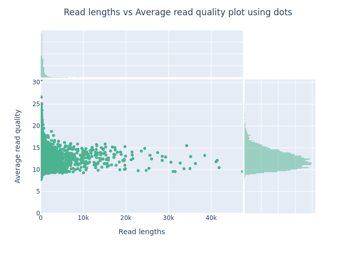
This is an example of a plot you might get from NanoPlot. Looking at plots like this helps you estimate how much data you’d lose by filtering on read quality or length.
- The top plot shows the frequency of read lengths
- The large main plot shows how read quality changes with read length
- The right plot shows the frequency of read qualities
Open the NanoPlot report for your sample.
Exercise 2 — interpret your plots
- How does the sequencing quality of your virome compare with the example image above? Cite specific metrics from your own NanoPlot results.
- What is the mean read quality NanoPlot reports for your sample?
- Do we need to remove any reads from our data? Why (not)?
- How much data would be lost from each sample if we filtered at Q7? At Q12?
Choosing filtering parameters
There is no universal quality threshold that should always be used for Nanopore viromics data. A suitable threshold depends on:
- the quality of the sequencing run;
- the amount of sequencing data available;
- read lengths;
- the downstream analysis;
- computational resources.
For this course, we will use relatively strict filtering because we will assemble the reads tomorrow. Assembly is computationally expensive, and reducing the number of reads makes the exercise faster and more manageable.
Open the supplied Chopper sbatch script. Using the Chopper documentation as a reference, adapt the script so it retains reads with a quality score of at least 24, a minimum length of 1000 and a maximum length of 40000.
Save the script and submit the job.
Check the .err and .out files to see if it ran successfully.
Exercise 3 — filter your reads
- How many reads do you have left after filtering?
How many reads were removed? Run NanoPlot again on the filtered reads to visualise the difference in read statistics. To do this, you need to change the
datadirandoutdirvariables in the existing script.- What is the average read quality before and after filtering?
Optional Challenge: Exploring GC content
If you have time left after filtering your reads, here’s an optional way to explore your data further.
So far we’ve filtered on read quality and length. There’s another useful signal worth checking: GC content: (sum of G’s + C’s) / (sum of all bases). There’s no universally “correct” GC content. Instead, it tells you something about the nucleic acid composition of your sample.
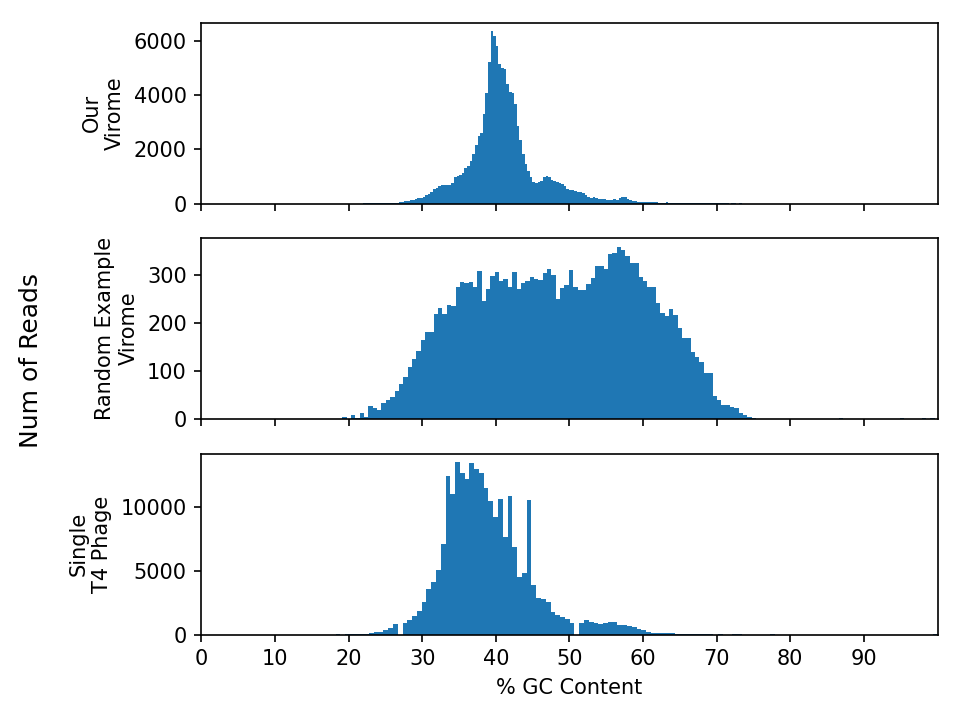
GC content is generally consistent along the length of a single genome. That means if you plot the GC content from reads coming from one genome in a histogram, you’d expect a unimodal distribution. Outlier regions within a genome (a horizontally transferred gene, an inserted prophage, a mobile genetic element) show up as reads that deviate from that peak.
Predicting the GC distribution of a virome
Before running the analysis discussion this question with a neighbour:
What do you expect the GC-content distribution of a virome to look like, compared to the GC-content distribution of a single genome?
Draw or describe your prediction and explain your reasoning.
Only after you made your prediction, use 1.1_40_gc_challenge.sbatch to plot the GC content of one of your fastq.gz files. You may need to update the read_path arguemnt to point to your fastq.gz file. The output should be in30_gc_content/gc_content.png. Use the VS Code Explorer to view your plot. If you want to make plots of multiple fastq.gz files, make sure not to override the output file :)
Questions
- Does your virome’s QC-content distribution match your prediction?
- Compare your plot with the example viromes and E. coli phage T4 genome provided below. Where does your sample fit?
- How would the GC content profile of a metagenome (bacteria and phages together) differ from a virome?
Resources
- Information about Nanopore sequencing quality and Phred scores
- How to write a for-loop to loop through your files
Key Points
Assembly lecture
Overview
Teaching: 120 min
Exercises: 60 minObjectives
Watch the lecture videos and read about assembly algorithms

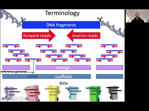
Sequence assembly is the reconstruction of long contiguous sequences (called contigs or scaffolds, see video below) from short sequencing reads. Before 2014, a common approach in metagenomics was to compare the short sequencing reads to the genomes of known organisms in the database (and some studies today still take this approach). However, this only works if the organisms in the database are closely related to the ones in the metagenomic sample. Recall that most of the sequences in a metavirome are unknown (“viral dark matter”), meaning that they yield no matches when compared to the reference database. Because of this, we need database-independent approaches to reconstruct new viral sequences. As sequencing technology and bioinformatic tools improved, sequence assembly enabled the recovery of longer sequences from metagenomic data. Having a longer sequence means having more information to classify it, so using metagenome assembly helps to characterize complex communities.
Video on sequence assembly
Watch the lecture video “Assembly strategies for genomics and metagenomics”. It will introduce reference-guided and de-novo assembly of genomic and metagenomic sequences (56 minutes):
Discussion
Watch the lecture video below and write down at least 3 questions and/or discussion points about it.
- Click on the image to see lecture video “Assembly strategies for genomics and metagenomics” by Prof Bas E. Dutilh (56 minutes):
Questions
- Would you use DBG (De-Bruijn Graph) or OLC (Overlap-Layout-Consensus) to assemble a dataset consisting of one billion short sequencing reads?
- What are the strengths and weaknesses of reference-guided assembly and de novo assembly?
- Would you use reference-guided or de novo assembly to assemble the genome of a model organism to discover mutations that occurred during an evolutionary experiment?
- Would you use reference-guided or de novo assembly to determine the genome sequence of an unknown organism?
- Why does metagenome assembly generally yield shorter contigs than genome assembly?
Conceptual questions
- What is the purpose of assembling sequencing reads? What information do assembled contigs provide that individual reads do not?
- What factors can make assembly of a virome difficult? Consider read quality, sequencing depth, genome diversity, and repeated or similar sequences. Connect this back to what you learned yesterday about read quality. How would systematic errors show up in an assembled contig? How would random errors show up?
Optional reading: Computational Biology: Genomes, Networks, Evolution MIT course 6.047/6.878 (Prof. Manolis Kellis). This book is part of a course on Computational Biology and contains several topics that are relevant for Bioinformatics. “5.2 Genome Assembly I: Overlap-Layout-Consensus Approach” and “5.3 Genome Assembly II: String graph methods” (pages 93 to 102) deal with assembly, if you want more details.
Key Points
Sequence assembly can be used to assemble genomes from reads
Metagenome assembly generally yields shorter contigs than genome assembly
Assembly of a metavirome
Overview
Teaching: 30 min
Exercises: 210 minObjectives
Understand how metavirome assembly converts sequencing reads into longer genomic sequences and evaluate the quality and characteristics of an assembly.
In this lesson, you will assemble the metavirome using the tool Flye introduced in this article. To then get a first idea about the diversity of the viral sequences contained in it, we will use vclust to group sequences together based on their similarity. Flye was designed to work well with noisy long reads and for metagenomic samples. Since you work on Draco, everything even slightly computationally expensive will be run through slurm. Please organize all the following steps in one or more sbatch scripts, as you learned yesterday. Since every tool needs different resources, it is recommended to have a single script per tool. All code snippets presented here assume that you put them in an adequate sbatch script. The necessary resources are mentioned in the comments or descriptions.
Assembly of a metavirome
There are multiple ways in which you can assemble reads from multiple samples as we have in our experimental data. We can just combine all data we have (replicates and conditions), to increase the coverage per virus. This can often be beneficial if the sequencing depth is not deep enough in the individual samples. Alternatively, we can assemble each sample indivudally. This preserves differences between samples which could get lost otherwise. Here, we will focus on a single assembly of a single file.
Exercise - Use flye to assemble one sample
To run a single sample assembly, you can use flye and output the assemblies into the folder 10_results_assembly_flye:
# The assembly can require large amounts of memory and time, depending on the number of reads
# and the diversity of the virome we want to study. Since we reduced the number of reads
# specifically to get a quick assembly, we can use about 50GB of RAM and 20 cores.

flye --nano-hq /path/to/filtered_reads.fastq.gz --meta -t 10   # don't forget to update the path to your filtered reads!
Here you can find an overview over the possible parameters.
Flye can be used for single-organism assemblies as well as metagenomic assemblies, so we use
--meta. Your sequences were generated with the Nanopore MinION platform and filtered to contain only high quality reads, which is why we use the--nano-hqparameter.-tdefines how many threads Flye can use. With--genome-sizewe give Flye a rough estimate of the total amount of sequence we expect. In a metavirome this is not one genome but the summed size of the whole viral community, so the value is only an order-of-magnitude guess; Flye uses it to calibrate its internal coverage estimates.After you have finalized your sbatch script with the resource assignments and the completed commands, you can run it to submit the assembly as a job to the Draco. You can check the output of your script in the slurm log files which you can set with the sbatch parameters at the beginning of your script. Check both files. Often, the error output contains more than just errors, and this file is the more informative one.
#SBATCH --output=10_assembly_flye/slurm/assembly_flye.slurm.%j.out
#SBATCH --error=10_assembly_flye/slurm/assembly_flye.slurm.%j.err
Flye creates an assembly in multiple steps. You can read through the Flye log file that you defined with the
#SBATCH --error=parameter. Afterward, you can find a list of all assembled contigs with additional information in the fileassembly_info.txt, located in the Flye output folder.
- What do the columns
#seq_name,length,cov., andcircmean?- What are the longest and shortest contig lengths?
- What is the range of depth (coverage) values?
- How many circular contigs were assembled? How can circular genomes get assembled?
- What does this tell us about these sequences/viral community? Connect it to the biology, not just the assembly process.
sbatch script for the assembly
#!/bin/bash
#SBATCH --tasks=1
#SBATCH --cpus-per-task=20
#SBATCH --partition=standard
#SBATCH --mem=50G
#SBATCH --time=01:00:00
#SBATCH --job-name=assembly_flye
#SBATCH --output=10_assembly_flye/slurm/assembly_flye.slurm.%j.out
#SBATCH --error=10_assembly_flye/slurm/assembly_flye.slurm.%j.err

# run flye in metagenomic mode for de-novo assembly of viral contigs
# First, activate the conda environment which holds the flye installation on draco:
source /vast/groups/VEO/tools/miniconda3_2024/etc/profile.d/conda.sh && conda activate flye_v2.9.2

# set a data directory holding your samples in .fastq.gz format
datadir="../1.1_QC/20_chopper"

# single assemblies
# Run flye on all samples sequentially, save the results in separate folders named like the samples:

outdir="10_assembly_flye"

flye --nano-hq $datadir/condition2_filtered_reads.fastq.gz --meta --genome-size 10m --out-dir $outdir -t 20

conda deactivate
Estimating the sequence diversity in your assembly
Which viruses did we sequence now? Without further analysis, we only have a nucleotide sequence and corresponding abundance estimates from the assembly. In the next days we will go through several steps to characterize the sequences we assembled now in more detail. Now, as a first overview over the diversity of the sequences, we will cluster them at 95% Average Nucleotide Identify (ANI) over 85% of the length of the shorter sequence. These cutoffs are often used to cluster viral genomes at the species rank. This can be done with the tool vClust and results in both, clustering very similar complete viral genomes and grouping genome fragments along with similar and longer sequences.
Exercise - use vClust to find similar contigs
vClust outputs, among other things, cluster representatives which are the longest sequences within a cluster. We use this mode to get the information we need to to estimate the diversity of the virome we sequenced. You can play with the similarity cutoffs (and metrics) used for clustering to see how they affect the results. vClust needs to align all sequences to each other and can run heavily in parallel. Remember to put this step into a sbatch script again and assign around 30 cores and 20GB of RAM.
# vClust is a python script and can be run by simply calling it on draco
# you have to run it with python 3.9
vclust='python3.9 /home/groups/VEO/tools/vclust/v1.0.3/vclust.py'

$vclust prefilter -i 10_assembly_flye/assembly.fasta ...
$vclust align ...
$vclust cluster ...
After vClust ran successfully, you can use a Python script to analyze the clusters computed by vClust. To parse a tabular file in the format of CSV or TSV (comma- or tab-separated values), the Python package pandas can be used. If its not in your virtual environment, install it now.
Pandas can be used to analyze the output of vClust. Some interesting aspects of the clusters we can compute from the cluster assignments alone are the number of clusters and how large the clusters are.
import pandas as pd
import os
from collections import Counter

# read the tsv file generated by vClust
cluster_df = pd.read_csv('path/to/the/file.tsv', sep='\t')

# use python's Counter object to count the "cluster" column in the vClust output table
cluster_counter = Counter(cluster_df["cluster"])

# use the counter object to compute how many clusters there are and how large they are
...
Python script for analyzing cluster sizes
import os
import pandas as pd
from collections import Counter


vclust_results_path = '20_vclust/'

for results_file in ("clusters_tani_90.tsv", "clusters_tani_70.tsv", "clusters_ani_90.tsv"):
    # read the tsv file generated by vClust
    cluster_df = pd.read_csv(os.path.join(vclust_results_path, results_file), sep='\t')

    # use python's Counter object to count the "cluster" column in the vClust output table
    cluster_counter = Counter(cluster_df["cluster"])
    n_clusters = len(cluster_counter)
    largest_clusters = cluster_counter.most_common(10)

    # output number of clusters and the sizes of the largest clusters
    print(results_file)
    print(f"Number of clusters: {n_clusters}")
    print("\n".join([f"{mc[0]}: {mc[1]}" for mc in largest_clusters]))
sbatch script for running vclust
#!/bin/bash
#SBATCH --tasks=1
#SBATCH --cpus-per-task=32
#SBATCH --partition=short,standard
#SBATCH --mem=10G
#SBATCH --time=01:00:00
#SBATCH --job-name=vclust
#SBATCH --output=20_vclust/slurm/vclust.slurm.%j.out
#SBATCH --error=20_vclust/slurm/vclust.slurm.%j.err


vclust='python3.9 /home/groups/VEO/tools/vclust/v1.2.7/vclust/vclust.py'

indir='10_assembly_flye/'
outdir='20_vclust/'

$vclust prefilter -i $indir/assembly.fasta -o $outdir/fltr.txt
$vclust align -i $indir/assembly.fasta -o $outdir/ani.tsv -t 30 --filter $outdir/fltr.txt
$vclust cluster -i $outdir/ani.tsv -o $outdir/clusters_tani_90.tsv --ids $outdir/ani.ids.tsv --metric tani --tani 0.90 --out-repr
$vclust cluster -i $outdir/ani.tsv -o $outdir/clusters_tani_70.tsv --ids $outdir/ani.ids.tsv --metric tani --tani 0.70 --out-repr
$vclust cluster -i $outdir/ani.tsv -o $outdir/clusters_ani_90.tsv --ids $outdir/ani.ids.tsv --metric ani --ani 0.90 --out-repr

source ../py3env/bin/activate

python3 ../python_scripts/1.2_vclust_results.py

deactivate
Questions - Go through the results of vClust
vClust is a great tool to get a feeling for the diversity within your assemblies (or any kind of set of sequences).
- How many sequence clusters were found in your assembly and how many sequences were grouped in the largest one?
- How do the results depend on the choice of your metric (ANI, TANI, or GANI) and your cutoff values?
- Why might there be a few large clusters and many small clusters? Think of possible biological explanations.
- What do our clustering results suggest about the redundancy or diversity of sequences in the assembly?
Key Points
Flye can be used to assemble long and noisy nanopore reads from metagenomic samples.
Samples can be assembled individually and combined in a cross-assembly
vClust can be used to assess the diversity of sequences in your assembly
Visualizing the assembly
Overview
Teaching: 0 min
Exercises: 60 minObjectives
Understand the topology of the de-Bruijn graph
Understand how the presence of similar species in the sample affects the assembly
Contig length distribution
To get an idea about the quality of your assembly, i.e. the degree of fragmentation and potentially full length complete viral genomes, it is helpful to look at the distribution of the length of the generated contigs. We can discribe this distribution using some numbers derived from it, such as the minimum, maximum or median length and something called N50 or N90. These numbers are computed by concatenating all contings ordered by their length. The length of the contig sitting at 50% (or 90%) of the total length of all contigs combined this way, is called N50 (or N90). The QUAST program (Gurevich et al., 2013) can be used to compute these values and visualize the distribution of the contig lengths. The tool can additionally use a reference sequence to compare the assembly against for assessing its fragmentation. We do not have a reference and will use the basic analysis of Quast.
Exercise - Use Quast to compute the contig length distribution
Use the Quast program to visualize the distribution of the contig lengths. You will need to run it two times, once per assembly, and save the results to different folders (ie.
result_quast/cross_assemblyandresult_quast/single_assemblies). Quast does not need many ressources. Assigning 2 CPUs and 5 GB of RAM for sbatch should be enough.# create a folder for the assessment within todays folder $ mkdir 30_results_assessment_quast # Quast is already installed on the server. Its a python script located here: $ quast='python3 /home/groups/VEO/tools/quast/v5.2.0/quast.py' # run quast $ $quast -o 30_results_assessment_quast/cross_assembly /path/to/your/cross_assembly/assembly.fastaYou can get the results from the file
report.txtor copy the whole results folder to your computer and openreport.htmlin your local browser.
How fragmented is your assembly?
The distribution of contig lengths can already tell you a lot about the assembly. Combined with some prior knowledge about the sample you sequenced, we can use it as an indicator of the quality or completeness of the assembly.
- What would be 2 extreme cases of length distributions? (Something other than no contigs at all :))
- How do the numbers we computed fit into your expectations about the sample you analyzed?
sbatch script for running Quast
#!/bin/bash
#SBATCH --tasks=1
#SBATCH --cpus-per-task=2
#SBATCH --partition=short,standard,interactive
#SBATCH --mem=1G
#SBATCH --time=00:30:00
#SBATCH --job-name=quast
#SBATCH --output=30_quast/quast.slurm.%j.out
#SBATCH --error=30_quast/quast.slurm.%j.err

# Set some variables for the quast script on draco and the files to be analysed
quast='python3 /home/groups/VEO/tools/quast/v5.2.0/quast.py'
assembly='10_assembly_flye/assembly.fasta'
outdir='30_quast'

# run Quast to visualize the distribution of contig lengths
$quast -o $outdir/assembly $assembly
Optional: Paths in the de-Bruijn graph
We will use Bandage, a tool to visualize
the assembly graph. Bandage is difficult to run on a Windows computer. In the
releases section, follow the instructions
to download the most appropriate version, such as Bandage_Ubuntu-x86-64_v0.9.0_AppImage.zip.
To run it, unzip the file and call Bandage from the terminal like this:
# run Bandage
$ ./Bandage_Ubuntu-x86-64_v0.9.0.AppImage
In File > Load_graph, navigate to and load the file assembly_graph.fastg of
the cross-assembly. Then click Draw graph to visualize the graph. Note that
this graph has already been compacted by collapsing nodes that form linear,
unbranching paths into unitigs. Nodes in the graph are called edge_N (confusing name…)
with N being an integer. They often correspond to the final contigs in your assembly.
Bubbles and junctions
Open the file
assembly_info.txtcorresponding to the graph you are looking at. The N in the node names as displayed by Bandage corresponds to the number assigned to continuous paths in the de-Bruijn graph by Flye. The “graph_path” column holds this information for all contigs.
- What does an asterisk * mean?
- What do multiple occurrences of the same number mean?
Pick two components of the visualized de-Bruijn graph and explain their topology and information content.
- Are there bubbles and junctions?
- Can you relate the complexity of the visualized graph to the Flye command line parameters?
Key Points
Bandage can visualize the de-Bruijn graph
JBrowse2 can visualize genomic data like alignments and coverage
Identifying Viral Contigs I
Overview
Teaching: 120 min
Exercises: 180 minObjectives
Read the abstract and introduction of the geNomad paper and extract the problem the tool was built to solve
Follow and reconstruct how geNomad classifies a sequence
Explain the tool in your own words, in writing

Reading a Tool Paper: geNomad
Every tool you run in this course makes decisions about your sequences. If you cannot describe those decisions, you cannot interpret the output, defend it in a discussion, or notice when it goes wrong. Today we want to understand something about virus identification. How can we do that only based on the assembled contigs we have now? In this theoretical part, we will try to make reading a tool paper closely enough to understand what the tool actually does a bit more fun by doing it together at the smart board.
Today we will read the paper: “Identification of mobile genetic elements with geNomad” (Camargo et al., 2023). geNomad identifies viruses and plasmids in sequencing data, assigns taxonomy to the viruses it finds, and annotates their genes. And it does this by combining two rather different ideas about what makes a sequence “viral”.
The session has three parts:
- Read on your own. Read the abstract and the introduction.
- Work through it together. We will then reconstruct how geNomad works at the board, step by step, until everyone feel like they can explain how the tool works in half a page.
- Write it down. Half a page.
Questions to read with
What problem do the authors say existing tools have? What is geNomad supposed to do better, and for whom?
geNomad identifies mobile genetic elements, not only viruses. What are mobile genetic elements, and why might it make sense to look for viruses and plasmids with the same tool?
The abstract mentions two very different sources of information used for classification. What are they? What kind of signal does each one capture, and where do you expect each to fail?
Note down terms and concepts in the abstract and introduction that are new to you.
Write-up
After the board session, write about half (!) a page covering:
- How geNomad decides whether a sequence is a virus, a plasmid, or neither.
- What you learned, things you didn’t know before.
- One thing you still do not understand.
Have fun :)
Key Points
geNomad combines two independent branches: an alignment-free model that reads the nucleotide sequence directly, and a gene-based model that uses marker protein profiles
Going through a paper together at the board is fun. Jeroen is amazing at drawing :)
Identifying Viral Contigs II
Overview
Teaching: 0 min
Exercises: 180 minObjectives
Identify phage contigs in an assembled virome
Interpret geNomad’s output
Assess assembly completeness
Select medium-complete and low-contaminated contigs
Select viral contigs for further analysis
In this section, we will identify viral sequences among our assembled contigs. We will use geNomad, which identifies both viruses and plasmids by combining a gene-marker classifier with a neural network operating on the nucleotide sequence. geNomad also assigns a taxonomy to the sequences it calls viral, so we will test how well it performs ourselves by running it on our virome contigs.
Identify viral contigs
We will start to identify viral contigs with geNomad.
Challenge
- Why is it important to use tools like geNomad on viromes?
Note that geNomad needs quite some memory to run, so allocate at least 20 GB for the sbatch job. Allocate 10 threads. geNomad runs on ordinary CPU nodes, so in the parameter --partition of the sbatch script you can use short,standard; no GPU allocation is needed. geNomad should run in a few minutes on our dataset.
Exercise
Run geNomad using the assembly as input:
- Read and interpret the output following geNomad’s quickstart page
source /vast/groups/VEO/tools/miniconda3_2024/etc/profile.d/conda.sh
conda activate genNomad_v1.11.2
genomad end-to-end -t 20 <assembly> <output_directory> /veodata/03/databases/geNomad/v1.11.2/genomad_db
geNomad writes its results into several subfolders of the output directory. The summary we will work with is
<outdir>/assembly_summary/assembly_virus_summary.tsv, which lists one row per sequence that geNomad classified as viral, together with its length, topology, virus score, number of hallmark genes and taxonomy. The corresponding sequences are inInspect the output files after running geNomad, and answer the questions below. ```bash head <output>
sbatch script for geNomad
#!/bin/bash
#SBATCH --tasks=1
#SBATCH --cpus-per-task=10
#SBATCH --partition=short,standard
#SBATCH --mem=20G
#SBATCH --time=2:00:00
#SBATCH --job-name=genomad
#SBATCH --output=10_genomad/genomad.slurm.%j.out
#SBATCH --error=10_genomad/genomad.slurm.%j.err

# this will run very quickly

source /vast/groups/VEO/tools/miniconda3_2024/etc/profile.d/conda.sh && conda activate genNomad_v1.11.2

# geNomad needs three positional arguments: the input assembly, the output
# directory, and the path to the geNomad database.
assembly='../1.2_assembly/10_assembly_flye/assembly.fasta'
outdir='10_genomad'
database='/veodata/03/databases/geNomad/v1.11.2/genomad_db'

genomad end-to-end -t 20 $assembly $outdir $database
Questions
- Do the results corroborate your expectations?
Was a contig classified as not viral? Take one of these contigs from the dataset and BLAST it using blastn. What are the top hits? Are they expected?
- How many viral contigs are there in the virome?
bash command for getting the number of phage contigs
geNomad’s virus summary contains only the sequences it called viral, so the number of viral contigs is simply the number of data rows in that file (the first line is a header):
tail -n +2 10_genomad/assembly_summary/assembly_virus_summary.tsv | wc -lTo see how the whole assembly was split between chromosome, plasmid and virus, use the aggregated classification instead:
cut -f 2- 10_genomad/assembly_summary/assembly_aggregated_classification.tsv | head
Estimating genome completeness
There are tools to assess the completeness of bacterial and viral genome sequences. For viruses we use CheckV. The tool identifies genes on the query sequence and compares them to a database of viral and bacterial marker genes. Each taxonomic group of bacteria or phages, e.g. a species or a family, has certain marker genes on its genome. So based on the number and types of marker genes, CheckV can figure out to which taxon a query contig belongs to and estimates how much of the genome it represents (estimated completeness). Note that, we will improve the taxonomic annotation in the “Viral Taxonomy and Phylogeny” section next week. CheckV also checks for unexpected marker genes on the sequence (estimated contamination), and whether part of a phage contig likely represents bacterial sequences, in which case the fragment could be part of a host genome with an integrated prophage.
Allocate 20 threads and at least 20 GB memory for the sbatch job. It should take ~1 minute to run.
# create a folder for the assessment (or let sbatch create it when you assign the output and error log files)
$ mkdir 20_results_assessment_checkv

# activate the conda environment containing the checkv installation
$ source /vast/groups/VEO/tools/anaconda3/etc/profile.d/conda.sh && conda activate checkv_v1.0.1

# run checkV on both assemblies
$ checkv end_to_end ...
sbatch script for running checkV
#!/bin/bash
#SBATCH --tasks=1
#SBATCH --cpus-per-task=20
#SBATCH --partition=short,standard
#SBATCH --mem=20G
#SBATCH --time=02:30:00
#SBATCH --job-name=checkv
#SBATCH --output=20_checkv/checkv.slurm.%j.out
#SBATCH --error=20_checkv/checkv.slurm.%j.err

# run CheckV to assess the completeness of single-contig virus genomes.
# First, activate the conda environment which holds the CheckV installation on draco:
source /vast/groups/VEO/tools/anaconda3/etc/profile.d/conda.sh && conda activate checkv_v1.0.1

# CheckV parameters (https://bitbucket.org/berkeleylab/checkv/src/master/#markdown-header-running-checkv)
# checkv end-to-end runs the CheckV pipeline from end to end :). It expects an input fasta file
# with the assembly and an output path.
# -t: threads

# assigning variables for readability

database='/veodata/03/databases/checkv/v1.5'
outdir='20_checkv'
assembly='../1.2_assembly/10_assembly_flye/assembly.fasta'

checkv end_to_end -t 20 -d $database $assembly $outdir
Go through the CheckV results
CheckV produces many output files, and also saves files for the intermediate steps of the tools that are used to find viral marker genes (diamond and hmmsearch). A summary of all results can be found in the file
quality_summary.tsv. Open the file and familiarize yourself with the information presented in the table. On CheckV’s website, you can find information about the output in the sections “How it works” and “Output files”.
- How are completeness and length related? (qualitative answer, name examples)
- What are possible reasons for contigs with low completeness to appear in the assembly?
Filter contigs
Exercise - select high-quality phage contigs
Use geNomad’s virus predictions and CheckV’s estimates of completeness and contamination to separate phage from non-phage contigs and reduce our assembly to high-quality contigs of high completeness. If you are an experienced programmer and have enough time, write (a) script(s) for that. If not, use the solutions below directly. For the solutions below, we used the file
assembly_virus_summary.tsvfrom geNomad’s summary folder, which already contains only the sequences classified as viral. The results of CheckV are located in the filequality_summary.tsvlocated in CheckV’s output folder.As a rule of thumb, you could keep all contigs with completeness >50% and contamination <5%. These values could be changed depending on the data and on the project. Note that filtering for low completeness can remove some conserved regions. Allocate 2 threads and 1GB memory for this job. It should take only a few seconds to run.
Note that geNomad renames sequences in which it detected a provirus: such a row has a
seq_namelikecontig_1|provirus_1200_15600instead ofcontig_1. Strip everything from the|onwards to get back the original contig name, otherwise those contigs will never match the CheckV table.To read the tabular files, you can use python’s pandas package. Then, you can load a .tsv file and select content from it like this:
import pandas as pd

# the .tsv format separates cells by a tab ('\t')
genomad_df = pd.read_csv(genomad_results_path, sep='\t')

# every row in the virus summary is a viral prediction; split off the provirus suffix
genomad_selection = {row['seq_name'].split('|')[0] for index, row in genomad_df.iterrows()}

# do the same for the checkv results and use set operations to get the contigs selected by both tools
joint_selection = genomad_selection.intersection(checkv_selection)

# modify the code from yesterday (rename and filter contigs) to go through the assembly and save contigs in the joint selection
...
python script for selecting viral contigs
import os, sys
import pandas as pd
from Bio import SeqIO

def main():

    assembly_path = os.path.abspath(sys.argv[1])
    assert assembly_path.endswith(".fasta")

    genomad_results_path = os.path.abspath(sys.argv[2])
    assert genomad_results_path.endswith(".tsv")

    checkv_results_path = os.path.abspath(sys.argv[3])
    assert checkv_results_path.endswith(".tsv")

    out_fasta = os.path.abspath(sys.argv[4])
    assert out_fasta.endswith(".fasta")

    # read the tsv files as pandas dataframes
    genomad_df = pd.read_csv(genomad_results_path, sep='\t')
    checkv_df = pd.read_csv(checkv_results_path, sep='\t')

    # collect the sets of contigs which stick to our selection cutoffs
    genomad_selection = {row['seq_name'].split('|')[0] for index, row in genomad_df.iterrows()}
    checkv_selection = {row['contig_id'] for index, row in checkv_df.iterrows() if row['completeness'] > 50 and row['contamination'] < 5}

    # use set operation union to get the contigs in the geNomad set AND in the checkv set
    joint_selection = genomad_selection.intersection(checkv_selection)

    # print some numbers
    print(f"Predicted viral contigs: {len(genomad_df.index)}, selected by geNomad: {len(genomad_selection)}, selected by checkv: {len(checkv_selection)}, joint selection: {len(joint_selection)}")

    # define list of records to keep and fill it by comparing the contig id of each record to the joint set of selected contigs
    out_records = []
    with open(assembly_path) as handle:
        for record in SeqIO.parse(handle, "fasta"):
            if record.id in joint_selection: out_records.append(record)

    # write the selected records into a new file
    with open(out_fasta, "w") as fout:
        SeqIO.write(out_records, fout, "fasta")

if __name__ == "__main__":
    main()
sbatch script for submitting the python script
#!/bin/bash
#SBATCH --tasks=1
#SBATCH --cpus-per-task=2
#SBATCH --partition=short
#SBATCH --mem=1G
#SBATCH --time=00:30:00
#SBATCH --job-name=filter_contigs
#SBATCH --output=30_filter_contigs/filter_contigs.slurm.%j.out
#SBATCH --error=30_filter_contigs/filter_contigs.slurm.%j.err

# activate the python virtual environment with the packages we need
source ../py3env/bin/activate

# in this sbatch script, its not necessarry to create the directory,
# we already told sbatch to create it for the log files.
# mkdir -p 30_results_filter_contigs

# In this solution, our script takes the assembly and the files
# 'assembly_virus_summary.tsv' from geNomad and
# 'quality_summary.tsv' from CheckV as an input. Set them as variables
# for readability
assembly='../1.2_assembly/10_assembly_flye/assembly.fasta'
genomadresults='10_genomad/assembly_summary/assembly_virus_summary.tsv'
checkvresults='20_checkv/quality_summary.tsv'
outdir='30_filter_contigs'

# run our script for filtering contigs based on the output of geNomad
# and CheckV as well as the output path.
python ../python_scripts/1.3_filter_contigs.py $assembly $genomadresults $checkvresults $outdir/assembly.fasta

# deactivate the environment
deactivate
Compare the results
CheckV and geNomad follow slightly different approaches, and we expect their outputs not to match perfectly. How different are their predictions?
At the selected cutoffs, how many contigs get chosen by geNomad, how many by CheckV?
How many geNomad hits were annotated by CheckV as having high-quality?
To find how many geNomad hits were annotated by CheckV as high quality:
tail -n +2 10_genomad/assembly_summary/assembly_virus_summary.tsv | cut -f1 | cut -d'|' -f1 | sort -u > phage_contigs_genomad.list

grep -w -Ff phage_contigs_genomad.list  20_results_assessment_checkv/cross_assembly/quality_summary.tsv | grep "High-" | wc -l
Key Points
Filtering contigs by completeness and contamination is crucial to obtain an informative dataset
Tools like geNomad classify your contigs, enabling you to understand your samples
No wet-lab or dry-lab technique is perfect. Filtering non-viral contigs from your data improves its quality, helping you obtain better results
Gene Calling and Functional Annotation I
Overview
Teaching: 180 min
Exercises: 60 minObjectives
Understand what gene calling and functional annotation are, and how together they turn a raw viral genome sequence into an interpretable one
Explain what ORFs are, describe phage-specific genomic features that make gene calling harder, and how tools like Phanotate are designed to handle them
Describe three complementary strategies for functional annotation (Pharokka, Phold and Phynteny)
Explain why these different strategies are required for functional annotation.

From assembled contigs to interpretable viral genomes
We have now identified viral contigs in our metagenomic data. But a DNA sequence by itself tells us very little about that virus. In this lesson, we will learn how to turn a (putative) viral genome sequence into an annotated genome.
This involves two main steps:
-
Gene calling: predicts the coordinates and strand of likely genes and their corresponding protein sequences.
-
Functional annotation: predicts what those proteins might do based on comparisons with known proteins and other sources of evidence.
The resulting information can then be presented in a gene table or as a genome figure, providing a more interpretable view of the viral genome.
In this lesson, you will learn about the principles behind gene calling and functional annotation. You will then apply these concepts in a practical annotation exercise.
Gene calling
The first step in annotating a viral genome is to identify where the genes are located.
Exercise
- What is the difference between an ORF and a gene?
- Why do we need specialised gene callers for phages?
- Name 3 features of phages that make gene calling challenging.
- Briefly describe the main idea behind the Phanotate algorithm.
- Malte and Jeroen made a new gene calling program called AwesomeGeneCaller. They ran Phanotate and AwesomeGeneCaller on a few viral genomes and compared the results. AwesomeGeneCaller predicts ten times more genes per viral sequence than Phanotate. Should Malte and Jeroen be happy? Why or why not?
Use the resources below to answer the questions. You are free to decide which resource(s) you use for each question. You do not need to use all of them.
-
Lecture (~18 minutes). This lecture by Dr. Robert Edwards gives an introduction to phages and discusses Phanotate, a gene-calling program developed in his lab. Stop at 18:14, when the lecture moves on to functional annotation.
-
Research paper: The phanotate paper describes the motivation and algorithm behind Phanotate.
-
This video by Dr. Katelyn McNair, the main developer of Phanotate, provides a more detailed explanation of how the algorithm works.
Functional annotation
Once we have identified the genes in a phage genome, we would like to know what those genes might do. This process is called functional annotation and can provide insights into phage biology, including its lifestyle, interactions with its host, and other potential functions encoded in its genome.
Note: For clarity we treat gene calling and functional annotation as two separate steps. In practice they are often performed together by a single tool. For example, Pharokka performs both gene calling (using Phanotate) and functional annotation.
In this part of the lesson, you will learn about three tools that use different types of evidence to predict the functions of phage proteins: Pharokka, Phold, and Phynteny.
You will first learn how these approaches work by reading parts of the corresponding papers. You will then use the Phage Annotation Server, which runs these three tools together, to annotate your own viral contigs.
1. Sequence-based annotation with Pharokka
Read Sections 1–2.4 of the Pharokka paper.
Answer the following questions:
Exercise
- What does Pharokka do, and which steps of the genome annotation process does it perform?
- What genomic features are taken into account when predicting genes?
- How does Pharokka assign functional annotations to predicted proteins?
- What is an HMM? Why are they useful for annotating phage proteins? What is a PHROG?
The PHROG paper and PHROGs database can be used as additional resources.
2. Phold
Sequence similarity is not the only source of information that can be used to predict protein function. Phold uses a different approach.
Read the abstract and introduction of the Phold paper, and/or watch this short video (5:53 min) where Phold is briefly explained.
Exercise
- Why might a sequence-based approach fail to assign a function to some phage proteins?
- What is the basic idea behind Phold?
- Why can Phold predict the function for more proteins than Pharokka?
3. Phynteny
Finally, read the abstract and introduction of Phynteny paper, to answer the following questions:
Exercise
- What is meant by synteny?
- How can Phynteny predict the function of a gene, when Phold and Pharokka cannot?
Key Points
Genome annotation gives meaning to genomic sequences
ORFs can be predicted from start and stop codons in the genomic sequences
Phages have different genomic features than prokaryotes, which influences the design of algorithms
Gene calling predicts the coordinates, strand, and protein sequence of candidate genes
Phage genomes have distinctive features (e.g. dense/overlapping genes, atypical start codon usage) that differ from prokaryotic genomes, requiring specialized tools like Phanotate
Sequence-based annotation (e.g. Pharokka) assigns function by comparing predicted proteins against known viral genes
Sequence similarity alone often fails on divergent phage proteins.
Gene Calling and Functional Annotation II
Overview
Teaching: min
Exercises: 240 minObjectives
Apply gene calling and functional annotation tools (Pharokka, Phold, Phynteny) to a real viral contig from your own assembly via the Phage Annotation Server
Compare how much each tool contributes to annotating a genome
Recognize why a large fraction of viral genes remain unannotated, even with modern tools
https://phage-annotation.org/jobs/34f6a6bdcbe64feea87639664a229ede/results
Choose a pet contig
In the previous lesson you learned about gene calling, and how Pharokka, Phold, and Phynteny use different approaches to annotate viral genes. Now you’ll apply all three to a contig from your own assembly.
Based on yesterday’s CheckV results, select a viral contig from your assembly that is either estimated High-quality or Complete. The TAs will help you coordinate so that everyone will work on a different contig.
The filtered viral sequences can be found in Viromics2026_workspace/1.3_virus_identification/30_filter_contigs/assembly.fasta
Exercise — extract your contig
- Use
1.4_10_select_contig.sbatchto extract a single contig from your filtered assembly. Fill in your assigned contig ID and submit it.The Phage Annotation Server is a website, so you’ll need the fasta file on your own laptop, not just on Draco.
In the VS Code Explorer, right-click on your extracted fasta file and select Download. Put somewhere you can find it on your laptop (e.g. your Downloads folder).
Alternatively, you can open the fasta file containing the filtered viral sequences you created yesterday, and copy and paste the sequence to a text file on your own computer.
If you found 20 or less viral sequences in your sample in the previous day, you can submit all viruses tpo phage-annotation.org (i.e. the complete
Viromics2026_workspace/1.3_virus_identification/30_filter_contigs/assembly.fastafile.
You can check how many contigs are in this file with:
cat Viromics2026_workspace/1.3_virus_identification/30_filter_contigs/assembly.fasta | grep ">" | wc -l
Annotate your contig
Exercise — submit for annotation
- Go to www.phage-annotation.org and upload your virus(es).
- Leave every option on its default setting and submit.
- Supply an email address so that you’ll receive an update. The typical turnaround is a few minutes, depending on queue load.
Predict before you look
While you wait: roughly what fraction of your contig’s genes do you expect Pharokka alone (sequence-based) to confidently annotate? Do you expect Phold and Phynteny to meaningfully increase that number? Why or why not, given what each tool actually uses as evidence?
Now look at the output from the phage-annotation website. You might want to download the results, and use Excel, R, or Python to answer the following questions:
Exercise — interpret your annotation
- How many genes were called on your contig in total?
- How many were annotated by Pharokka’s sequence-based search alone? How many additional genes did Phold and/or Phynteny resolve? Does this match your prediction above? Look at the figure on the Phynteny website. Does this match your results?
- Identify at least 2 structural genes (e.g. capsid, tail, portal). Where are they in the genome, and which tool provided the evidence for each?
- Identify one replication-associated gene. What’s its function, and where in the phage life cycle is it used?
- Note any other interesting features (CRISPR arrays, tRNAs, anti-CRISPR genes, auxiliary metabolic genes).
- Based on everything above, what can you infer about this virus’s lifestyle (lytic vs. temperate) and its likely interaction with a host?
- Look at the genome organisation. Describe what you see. Look for genes annotated by Phynteny but not any of the other tool. Do you notice anything particular?
Interpret your results
You’ll find that most genes on viral contigs are not actually annotated. There are several reasons:
- Rapid evolution: Viruses can evolve rapidly, making homology-based annotation genuinely difficult. A gene may diverge beyond the point where detectable sequence similarity is possible.
- Highly mosaic genomes: Phages frequently acquire and lose genes from their hosts and from other phages. As a result, related viruses can have very different gene complements, and reference databases do not fully capture this diversity.
- Limited characterisation of viral sequence space: A large fraction of viral diversity remains unexplored. A hypothetical protein annotation is therefore not necessarily a failure of the annotation tools, instead it reflects how little of viral sequence space has been characterised.
Finally, download your phage-annotation.org results from the website. You will need these tomorrow
(Press the ‘Download all (.zip file) button in the top right corner.)
Key Points
Most genes on viral contigs remain unannotated due to rapid viral evolution, highly mosaic genomes, and how little of viral sequence space is characterized in reference databases
Using structure-based search or genomic context can be used to detect distant homologies, allowing for the annotation of more viral genes.
Viral taxonomy and phylogeny I
Overview
Teaching: 60 min
Exercises: 120 minObjectives
Understand the differences between taxonomic approaches for viral and cellular organisms
Explain the challenges with viral taxonomy, and how they may be overcome

Brief introduction on viral taxonomy
There is no single method to classify the taxonomy of viruses. Many experts from the global virology community have done their part by classifying viruses according to their specific knowledge. This has generated a patchwork of methods that capture the features of different viral lineages and generate meaningful taxa that are in agreement with biology. With the advancement of viromics and the discovery of viruses by their genome sequences only, new methods are necessary to classify viruses based on their sequences, similar to approaches for cellular organisms.
A widely accepted approach for sequence-based taxonomic classification is by selecting a marker gene that is shared by all organisms, creating a multiple sequence alignment and phylogenetic tree, and identifying taxa as characteristic branches or lineages in the tree. This approach can be applied to all cellular organisms including bacteria, archaea, and eukaryotes, particularly using with ribosomal genes such as 16S small subunit in prokaryotes or the 18S in eukaryotes. As no marker gene is universally conserved in all viruses, this approach is only possible in subgroups of viruses. The lack of a universal genomic feature is thought to reflect their multiple evolutionary origins.
Bioinformaticians have developed many methods to circumvent the lack of a universal gene, for example, by cluster viral sequences. However, so far these methods have not been widely adopted for official ICTV virus taxonomy.
One popular method in the bacteriophage field is the gene-sharing network. This involves creating a network where nodes are viral genomes and edges represent shared gene families between these genomes. Tight clusters in this gene-sharing network represent groups of viral genomes that share many genes, and those could be interpreted as taxonomic groups. Networks can be built with different gene-sharing cutoffs, corresponding to different taxonomic ranks, where closely related viruses (species, genera) share more genes than distant ones (families). Tools like VICTOR and vConTACT3 work this way.
As more and more viruses are sequenced and we get a better view of the virosphere, marker genes are making a comeback. Although a universal marker gene shared by all viruses does not exist, marker genes are certainly shared by viruses of lower-ranking taxa (species, genera, families, orders, and in some cases above). Detecting the marker gene is evidence that a virus belongs to a given taxon, and phylogenetic trees can help resolve the lower-level taxonomy, just like ribosomal marker gene trees for cellular organisms. Tools like vClassifier and geNomad use marker gene approaches.
Exercise - Classifying viruses
Read the abstract, introduction and following sections from the review “Global Organization and Proposed Megataxonomy of the Virus World” by Koonin et al.:
- The Baltimore classes of viruses, virus hallmark genes, and major evolutionary trends in the virus world
- Evolutionary links among viruses within and across the Baltimore classes, section: Double-Stranded DNA Viruses
Discuss with your fellow students and write down your answers:
- What is the difference between a taxonomy and a phylogeny?
- What are the Baltimore Classes, and what are they based on?
- What would you like a taxonomy of viruses to reflect? i.e. what does a ‘good’ viral taxonomy describe?
- Does the Baltimore classes satisfy the previous question?
- What triggered the change in viral taxonomy?
- What makes it hard to make a good taxonomy of viruses? Name at least 2 points.
Exercise - The ICTV
Check out the ICTV website: https://ictv.global/.
Discuss with your fellow students and write down your answers:
- What is ICTV? (not just a TV channel featuring polar bears)
- How many taxonomic ranks are available to classify the virosphere?
- What is a realm?
- How many viral genera are there?
- Pick one marker gene and describe how it functions in the virus-host interaction, which taxonomic rank it can/cannot identify.
In the practical section of this day, we will be using marker gene methods to classify the viruses identified in our metaviromes. Examples of widely used marker genes are for phages include the terminase large subunit (terL), major capsid protein (mcp) and DNA polymerase B (PolB).
Key Points
Viruses have multiple origins, so there is no universal marker gene
Viral taxonomy is based on many different methods
Gene-sharing networks and marker genes are popular methods for bacteriophage taxonomy
Viral taxonomy and phylogeny II
Overview
Teaching: 210 min
Exercises: 0 minObjectives
Create a viral phylogeny based on the terL gene
What kind of phages exist in your dataset?
For this task, we will first build a phylogenetic tree using the terL marker gene.
TerL phylogenetic tree
The terminase large subunit is a widely used marker gene for phages. This protein packages the DNA into an empty pro-capsid. It has two parts: 1) an ATP driven motor for viral DNA translocation and 2) a endonuclease to cleave the viral DNA to signal the end of the packaging reaction, once the capsid is full. TerL is quite essential in the assembly of full icosahedral capsids, and therefore makes a good marker gene for the Caudoviricetes order. Consider also that some phages do not require, and therefore, do not encode a terL gene.
Basics of making a tree
- Start with amino acid sequences in a fasta file
- Make a multiple sequence alignment (MSA) - this identifies biologically informative positions for tree inference
- INSPECT your MSA - you might need to trim poorly aligned columns
- Build a tree - there are several tree building algorithms - we will use maximum likelihood
Exercise - Make a terL phylogenetic tree with your sequences
For this exercise, we will use the ICTV reference phages. We have extracted the terL amino acid sequences from the ICTV reference phages using pharokka, and pre-built a multiple sequence alignment. You will have to add your sequences to this alignment using mafft and then trim the alignments using trimAl and build a tree using FastTree 2. The solution sbatch script at the bottom of the tree-making section includes all the tree-making steps.
To get a fasta file of your terL amino acid sequences (output by Pharokka) and locate the pre-built MSA
# location of the terL sequences from pharokka output
./1.4_annotation/10_pharokka/terL.faa

# location of the reference pre-built MSA
/vast/groups/VEO/shared_data/Viromics2025_workspace/data/alignments/terL_ICTV_ref_phage_alignment.fasta

# copy the terL alignment to your own directory
mkdir -p viromics/data/alignments   # make a directory if it doesn't exist
cp /vast/groups/VEO/shared_data/Viromics2025_workspace/data/alignments/terL_ICTV_ref_phage_alignment.fasta viromics/data/alignments
To add your terL sequences to the reference alignment using mafft. You need the following command and it will take ~22min
/home/groups/VEO/tools/mafft/v7.505/bin/mafft --reorder --keeplength --addfragments contigs_terL.fasta reference_alignment.fasta > new_MSA.fastaTo trim your alignment using TrimAl (-gappyout)
trimal -in new_MSA.fasta -out new_MSA_trimmed.fasta -gappyoutTo build a tree using FastTree.
/home/groups/VEO/tools/fastTreeMP/v2.1.11/FastTreeMP -lg -pseudo < new_MSA_trimmed.fasta > new_MSA_trimmed.tree

# -lg : Uses the LG model. Note: the LG model is an updated model that describes how likely it is that one amino acid is replaced by another based on patterns found in real protein families. The default model for Fasttree is the JTT - which is older but similar model.
# -pseudo : Adds pseudo counts (for gappy alignments)
TerL tree outputs
Phylogenetic trees come in several output types but here the above commands produce a tree in a newick format. This is a text file and you can open it with any text editor to see what it looks like. It takes the shape: (A:0.1, B:0.2, (C:0.3, D:0.4)E:0.5)F;
The final terL tree might look something like this:
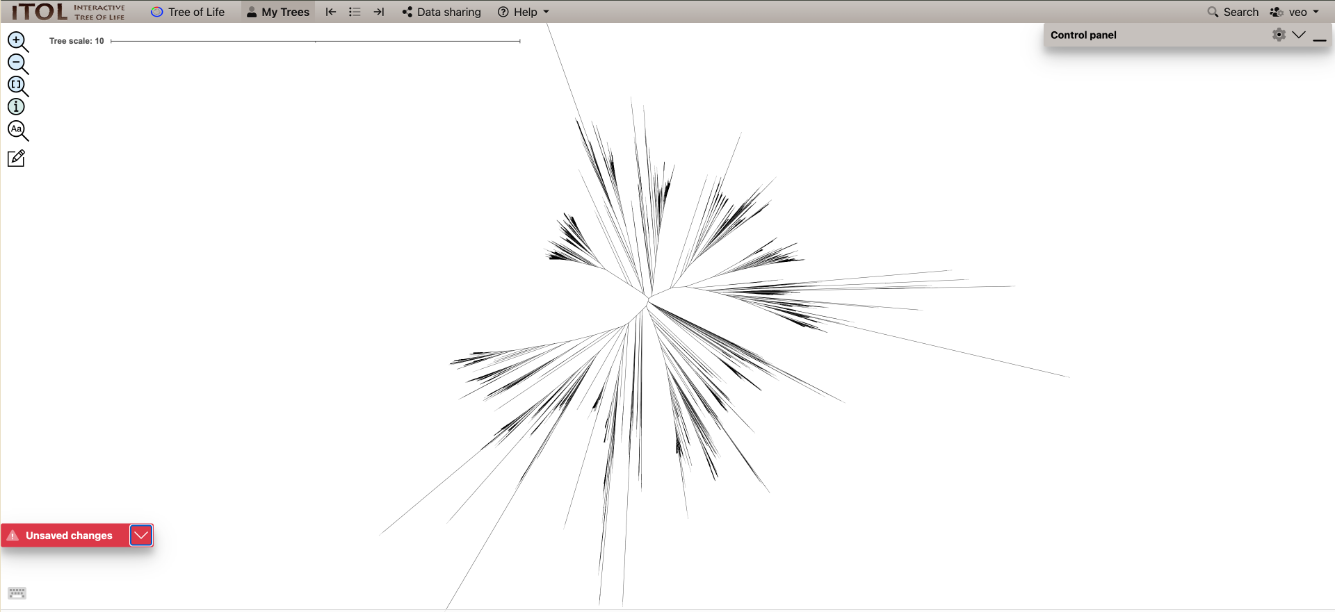
This .tree file can be opened with dendroscope (if you downloaded it locally) or iTOL or another tree-visualization software HOWEVER the full terL tree we will produce will have 5000+ leaves, which will be difficult to load into tree-viewers and might crash your computer when trying to find your viruses.
Instead, you could post-process the tree using the ete3 library in Python.
Exercise - Post-process large tree –> smaller tree
There are a few ways to post-process trees to make them viewable or to highlight our viruses of interest.
- One way would be build a script that takes the input of a single contig and the tree file and pruning the tree around the contig to a certain number of the closest reference viruses. Pruning a tree means only certain clades or leaves are left.
- Instead of pruning, you can also “collapse” clades to make the tree manageable to view. For this, clades are collapsed into a single leaf that replaces them. In very large trees, you will probably encounter large clades that are far away from your sequences of interest that can be collapsed and replace. For this, you might want to give an input of all your viruses of interest.
We’ve built two python scripts using this library to shrink the size of tree outputs. The locations of the tree-pruning scripts will be in your python_scripts directory python_scripts/1.5_collapse_non_target_clades.py and python_scripts/1.5_trim_tree_to_500_neighbors.py.
1.5_trim_tree_to_500_neighbors.py will trim your tree around a contig of your choice to the closest 500 neighbours. 1.5_collapse_non_target_clades.py will collapse clades that don’t contain viruses from our dataset. These scripts also include a section to generate ITOL annotation files.
python script to trim tree around 1 contig
# trim_tree_to_500_neighbors.py

from ete3 import Tree
import sys

def trim_tree(input_tree_file, target_leaf_name, output_tree_file, itol_output_file=None, num_neighbors=500):
   tree = Tree(input_tree_file, format=1)

   if not tree.search_nodes(name=target_leaf_name):
       raise ValueError(f"Leaf '{target_leaf_name}' not found in the tree.")

   target_leaf = tree&target_leaf_name
   leaves = [(leaf, target_leaf.get_distance(leaf)) for leaf in tree.iter_leaves()]
   leaves.sort(key=lambda x: x[1])

   # Get ~500 closest neighbors including the target leaf
   closest_leaves = set([leaf.name for leaf, dist in leaves[:num_neighbors]])

   # Prune the tree
   pruned_tree = tree.copy()
   pruned_tree.prune(closest_leaves, preserve_branch_length=True)
   pruned_tree.write(outfile=output_tree_file, format=1)

   if itol_output_file:
       user_colour = "#079907"       # Green for user nodes
       with open(itol_output_file, "w") as f:
           f.write("DATASET_SYMBOL\n")
           f.write("SEPARATOR TAB\n")
           f.write("DATASET_LABEL\tUser-selected leaves\n")
           f.write("COLOR\t#00cc00\n")
           f.write("DATA\n")
           f.write(f"{target_leaf_name}\t3\t2\t{user_colour}\t1\t1\n")      # symbol star=3, size=2, fill=1,position=1

if __name__ == "__main__":
   if len(sys.argv) not in (4, 5):
       print("Usage: python trim_tree_to_500_neighbors.py input_tree.nwk target_leaf_name output_tree.nwk [itol_output.txt]")
       sys.exit(1)
   itol_output = sys.argv[4] if len(sys.argv) == 5 else None
   trim_tree(sys.argv[1], sys.argv[2], sys.argv[3], itol_output)
python script to collapse clades except our viruses
# collapse_non_target_clades.py

from ete3 import Tree
import sys

def collapse_large_non_target_clades(input_tree_file, user_leaves_file, output_tree_file, itol_output_file=None, threshold=100):
   tree = Tree(input_tree_file, format=1)

   with open(user_leaves_file) as f:
       target_leaves = set(line.strip() for line in f if line.strip())

   collapsed_info = []
   node_counter = [1]

   def process_node(node):
       leaves_in_subtree = set(leaf.name for leaf in node.iter_leaves())
       if len(leaves_in_subtree) > threshold and not (leaves_in_subtree & target_leaves):
           collapsed_name = f"collapsed_node_{node_counter[0]}"
           node.name = collapsed_name
           node_counter[0] += 1
           collapsed_info.append((collapsed_name, len(leaves_in_subtree)))
           node.children = []
       else:
           for child in node.children:
               process_node(child)

   process_node(tree)

   tree.write(outfile=output_tree_file, format=1)

   if itol_output_file:
       # collapsed_colour = "#878787"  # Blue for collapsed nodes
       user_colour = "#079907"       # Green for user nodes

       # with open(itol_output_file, "w") as f:
       #     f.write("DATASET_TEXT\n")
       #     f.write("SEPARATOR TAB\n")
       #     f.write("DATASET_LABEL\tCollapsed Nodes\n")
       #     f.write(f"COLOR\t{collapsed_colour}\n")
       #     f.write("DATA\n")
       #     for node_name, size in collapsed_info:
       #         if not node_name:
       #             continue  # Skip blank node names just in case
       #         f.write(f"{node_name}\t{collapsed_colour}\tClade ({size} leaves)\n")

       # Write user leaf highlight using green stars (iTOL DATASET_SYMBOL)
       # highlight_file = itol_output_file.replace(".txt", "_user_symbols.txt")
       with open(itol_output_file, "w") as f:
           f.write("DATASET_SYMBOL\n")
           f.write("SEPARATOR TAB\n")
           f.write("DATASET_LABEL\tUser-selected leaves\n")
           f.write("COLOR\t#00cc00\n")
           f.write("DATA\n")
           for leaf in sorted(target_leaves):
               f.write(f"{leaf}\t3\t2\t{user_colour}\t1\t1\n")      # symbol star=3, size=2, fill=1,position=1

if __name__ == "__main__":
   if len(sys.argv) not in (4, 5):
       print("Usage: python collapse_non_target_clades.py input_tree.nwk user_leaves.txt output_tree.nwk [itol_output.txt]")
       sys.exit(1)
   itol_output = sys.argv[4] if len(sys.argv) == 5 else None
   collapse_large_non_target_clades(sys.argv[1], sys.argv[2], sys.argv[3], itol_output)
Exercise - Post-process your tree
Use the below sbatch script make your tree and post-process it. Note: For some exercises today, pick a pet contig (maybe the same as the one yesterday!). You will have change the contig name in the sbatch scripts accordingly.
Please pause once you have made the trees! We will visualize the tree together with a demo in itol so that you can make nice graphics to include in your lab books!
sbatch script to make tree and post-process it
#!/bin/bash
#SBATCH --tasks=1
#SBATCH --cpus-per-task=10
#SBATCH --partition=short,standard,interactive
#SBATCH --mem=50G
#SBATCH --time=2:00:00
#SBATCH --job-name=terL_tree
#SBATCH --output=./10_terL_tree/terL.slurm.%j.out
#SBATCH --error=./10_terL_tree/terL.slurm.%j.err

# Run mafft to add the sequences
mafft="/home/groups/VEO/tools/mafft/v7.505/bin/mafft"
new_seqs="../1.4_gene_annotation/10_pharokka/results/terL.faa"
terl_aln="../data/alignments/phylogenetic_alignments/terL_ICTV_ref_phage_alignment.fasta"

# have to add sequences to untrimmed alignment, since mafft doesn't know what was trimmed
$mafft --add $new_seqs --reorder $terl_aln > ./10_terL_tree/terL_MSA.fasta

# Trim the alignment using trimAl
trimal="/home/groups/VEO/tools/trimal/v1.5.0/trimal/source/trimal"
$trimal -in ./10_terL_tree/terL_MSA.fasta -out ./10_terL_tree/terL_MSA_trimmed.fasta -gappyout

# Build a tree using fasttree
fastTreeMP="/home/groups/VEO/tools/fastTreeMP/v2.1.11/FastTreeMP"
$fastTreeMP -lg -pseudo < ./10_terL_tree/terL_MSA_trimmed.fasta > ./10_terL_tree/terL_MSA_trimmed.tree

source ../py3env/bin/activate

# change your contig name here
contig_name=contig_71_CDS_0091

# prune the tree based on your selected contig
python3 ../python_scripts/1.5_trim_tree_to_500_neighbors.py ./10_terL_tree/terL_MSA_trimmed.tree $contig_name ./10_terL_tree/terl_${contig_name}_pruned.tree ./10_terL_tree/${contig_name}_itol_annotation.txt

# get all your viruses into user_leaves.txt
grep ">" ../1.4_gene_annotation/10_pharokka/results/terL.faa | sed 's/>//g' |sed 's/ .*$//' > ./10_terL_tree/user_leaves.txt

# collapse tree branches except user defined leaves
python3 ../python_scripts/1.5_collapse_non_target_clades.py ./10_terL_tree/terL_MSA_trimmed.tree ./10_terL_tree/user_leaves.txt ./10_terL_tree/terl_collapsed.tree ./10_terL_tree/collapsed_itol_annotation.txt

deactivate
Exercise - comparing your taxonomic annotations
- What is the taxonomy classification of your pet contig from the terL tree? (if at all)
Group Discussions
- Explore the terL tree together - include a graphic of at least 1 tree
- What do long branches on your terL tree mean?
- What does a rooted versus an unrooted tree represent?
- What are the limitations of using the terL tree? and could you overcome these limitations?
Hint on querying pickle files using python
import pandas as pd

# read in the shared genes pickle file
# this pickle file contains genes shared at even 30% identity - there are other files for 40, 50 ,60 and 70% identity
df_3 = pd.read_pickle("HMMprofile.0.3_SqRoot_shared_genes.pkl.gz")
df_3
# check how many genes contig_518 shares with the other contigs
df_3_contig_518 = df_3.loc[df_3['contig_518'] > 0, 'contig_518']
df_3_contig_518
Key Points
Marker genes such as the terminase large subunit (terL) can also be used to judge how related viruses are and in some cases classify the taxonomy as lower taxa ranks
Host Prediction I
Overview
Teaching: 60 min
Exercises: 120 minObjectives
Understand how biological information is used to predict hosts
Understand the difficulties with host prediction
Learn about the new techniques that are being used for host prediction

Host prediction lecture
We will start with a short lecture, then you can either read the abstract and introduction of the PhageTransformer preprint or the RaFAH paper. Both tools use a machine learning approach to solve the phage-host prediction problem. Please choose only one paper and afterwards we will discuss the differences.
Write a short summary
Please write half a page into your daily report about phage-host interactions and how we can predict them. You dont have to explain everything, you can focus on parts of what we went through. You can work along the following points:
- What are some biological interactions viruses have with their hosts?
- How can we exploit these interactions?
- There are many methods for predicting phage-host interactions. What are some of the issues they run into?
- How can you be confident in your host prediction?
Additional resources
- IBM link on Random Forest (RF): introduces RF and decision trees in a short and simple way
- Chapter on RF for Bioinformatics: explains how RF measures feature importance and describes Bioinformatic applications
- Chapter on Decision Trees and RF: describes decision trees and RF by direct application in python. Also, if you want a great introduction to machine learning in general and python programming, take a look at the whole book by Jake VanderPlas, which is freely available online
Key Points
Host Prediction II
Overview
Teaching: 0 min
Exercises: 300 minObjectives
Run RaFAH and PhageTransformer to predict a host genus for each contig.
Host prediction
Today, we will use the tools RaFAH and PhageTransformer to predict a genus of a putative host for our contigs. RaFAH predicts proteins in each viral sequence and then assigns them to a set of orthologous groups. The annotated proteins are then used to predict a host genus with a pretrained random forest model.
Next, we will use PhageTransformer as an alternative way of linking viruses to their hosts. PhageTransformer employs a genome language model to predict one or more hosts for a given input sequence. It can also identify bacterial sequences and gives you an additional estimate of how reliable a prediction is.
Finally, we will compare the resulting predictions and discuss the results together.
RaFAH
Exercise - Use RaFAH to predict hosts for our contigs
RaFAH requires a single file for each contig to run. You first have to write a python script which separates the combined assembly into single files. You can use the package biopython installed in your virtual environment for this:
import os, sys
from Bio import SeqIO

# define file paths from the arguments
...

# loop through the records in the combined assembly
with open(assembly_path) as handle:
    for record in SeqIO.parse(handle, "fasta"):
        # set a filename per record
        out_fasta = os.path.join(out_dir, f"{record.id}.fasta")
        # write the record to the file
        with open(out_fasta, "w") as fout:
            SeqIO.write([record], fout, "fasta")
You can run the script in the same sbatch script as RaFAH. Remember to source and deactivate our python virtual environment accordingly. Here you can find a description of the parameters you can pass to RaFAH (the page is a bit hard to read). The tool is programmed in perl and you can find it here on draco:
# activate the conda environment with the dependencies RaFAH requires
source /vast/groups/VEO/tools/miniconda3_2024/etc/profile.d/conda.sh && conda activate perl_v5.32.1

# set a variable to call the RaFAH script
rafah='/home/groups/VEO/tools/rafah/RaFAH.pl'

# create an output folder or use the one you set for the slurm logs:
mkdir 10_results_hostprediction_rafah

# run RaFAH with the appropriate file paths and arguments
perl "$rafah" --predict --genomes_dir 10_results_hostprediction_rafah/split_contigs --extension .fasta
RaFAH is computationally expensive and can use multiple threads. We recommend you set the following sbatch parameters:
- #SBATCH –cpus-per-task=20
- #SBATCH –partition=standard
- #SBATCH –mem=50G
RaFAH uses the random forest model to compute a probability for all host genuses included in its training. You can find these probabilities in the output file
*Host_Predictions.tsv. The file*Seq_Info_Prediction.tsvcontains per contig the genus with the highest probability.
- How many contigs have a high probability score and do you trust these predictions?
python script for splitting the assembly into separate files
import os, sys
from Bio import SeqIO

def main():

    # define file paths from the arguments
    assembly_path = os.path.abspath(sys.argv[1])
    assert assembly_path.endswith(".fasta")

    # set an output directory and create it if it does not exist
    out_dir = os.path.abspath(sys.argv[2])
    if not os.path.exists(out_dir): os.makedirs(out_dir)

    # loop through the records in the combined assembly
    with open(assembly_path) as handle:
        for record in SeqIO.parse(handle, "fasta"):
            # set a filename per record
            out_fasta = os.path.join(out_dir, f"{record.id}.fasta")
            # write the record to the file
            with open(out_fasta, "w") as fout:
                SeqIO.write([record], fout, "fasta")

if __name__ == "__main__":
    main()
sbatch script for host prediction with RaFAH
#!/bin/bash
#SBATCH --tasks=1
#SBATCH --cpus-per-task=32
#SBATCH --partition=standard
#SBATCH --mem=50G
#SBATCH --time=02:00:00
#SBATCH --job-name=rafah
#SBATCH --output=10_rafah/rafah.slurm.%j.out
#SBATCH --error=10_rafah/rafah.slurm.%j.err

assembly='../1.3_virus_identification/30_filter_contigs/assembly.fasta'
contigs='10_rafah/split_contigs'
mkdir -p "$contigs"

# RaFAH expects each genome in a separate file. Activate our virtual environment
# and run a python script to split our filtered assembly into single files
source ../py3env/bin/activate

# The script requires the assmbly path and a directory for outputting the contigs
python ../python_scripts/2.1_split_assembly.py $assembly $contigs

# deactivate the python environment, just to be sure not to cause problems with the conda environment RaFAH needs
deactivate

# activate the conda environment with the dependencies RaFAH requires
source /vast/groups/VEO/tools/miniconda3_2024/etc/profile.d/conda.sh && conda activate perl_v5.32.1

# set a variable to call the RaFAH script
rafah='/home/groups/VEO/tools/rafah/RaFAH.pl'

# rafah parameters (https://gensoft.pasteur.fr/docs/RaFAH/0.3/)
# --predict: run the pipeline for predicting hosts
# --genomes_dir: the directory with the separate files for each contig
# --extension: the extension of the contig files
# --file_prefix: can specify an output dir here and "run name" (rafah_1) here

perl "$rafah" --predict --genomes_dir $contigs --extension .fasta --file_prefix 10_rafah/rafah_1

# deactivate RaFAH's conda environment
conda deactivate
PhageTransformer
Exercise - Use PhageTransformer to predict hosts for our contigs
Unlike RaFAH, PhageTransformer takes the whole assembly as a single multi-fasta file, so no splitting step is needed. It reads the nucleotide sequences directly and does not depend on gene calling or protein annotation.
# activate the conda environment holding the PhageTransformer installation
source /vast/groups/VEO/tools/miniconda3_2024/etc/profile.d/conda.sh && conda activate phagetransformer_v0.2.1

# the pretrained model lives in its own directory on draco
model="/home/groups/VEO/tools/phagetransformer/v0.2.1"

# run the prediction; results are written to standard output, so redirect them into a file
phagetransformer predict --input <assembly> --model_dir $model > <output.tsv>
PhageTransformer is a language model and runs roughly 200x faster on a GPU than on CPUs. We recommend you set the following sbatch parameters:
- #SBATCH –cpus-per-task=4
- #SBATCH –partition=short,standard
- #SBATCH –mem=10G
Since we only have a handful of contigs, the job also finishes in reasonable time on an ordinary CPU node. If the GPU partition is busy, drop the
--gresline and use--partition=short,standardinstead.The output table contains one row per contig with the predicted host and a score expressing how confident the model is. PhageTransformer can also report that a sequence looks bacterial rather than viral, which is a useful sanity check on our filtered assembly.
- How many contigs get a host prediction, and how are the confidence scores distributed?
- Does PhageTransformer flag any of our contigs as bacterial? What would that mean for the filtering we did in the virus identification section?
sbatch script for host prediction with PhageTransformer
#!/bin/bash
#SBATCH --tasks=1
#SBATCH --cpus-per-task=4
#SBATCH --partition=standard
#SBATCH --mem=10G
#SBATCH --time=01:00:00
#SBATCH --job-name=pt
#SBATCH --output=./20_phagetransformer/slurm/phagetransformer.slurm.%j.out
#SBATCH --error=./20_phagetransformer/slurm/phagetransformer.slurm.%j.err

# source the conda env on draco, set model directory
source /vast/groups/VEO/tools/miniconda3_2024/etc/profile.d/conda.sh && conda activate phagetransformer_v0.2.1
model="/home/groups/VEO/tools/phagetransformer/v0.2.1"

# PhageTransformer takes the whole filtered assembly at once
assembly='../1.3_virus_identification/30_filter_contigs/assembly.fasta'
outtsv='20_phagetransformer/predictions.tsv'

# the tool writes its table to standard output, so we redirect it into a file
phagetransformer predict --input $assembly --model_dir $model > $outtsv

conda deactivate
Exercise - comparing RaFAH and PhageTransformer results
- For how many host predictions do RaFAH and PhageTransformer agree and upto which taxonomic level?
- How do you explain the differences between the predictions?
- Which predictions do we trust, how can we get more confident?
Key Points
RaFAH uses a random forest model to predict hosts to the genus level for phages
RaFAH returns a probability for each host genus it can predict.
PhageTransformer is a codon-aware genome language model that predicts a host from DNA sequence directly.
Designing a Research Project
Overview
Teaching: min
Exercises: 420 minObjectives
Develop a conceptual pipeline of analysis
Define a hypothesis based on your research question
Choose one or more papers for inspiration
Create a flow diagram (workflow or pipeline)
Plan to end your project with an ecological hypothesis
To close off this course, we would like to give you the opportunity to design your own research project. Viromics is a new field, the virosphere is huge, and there is a LOT of data, so there are more unanswered than answered questions. We thought of three projects, all inspired by the experiments done in the wet lab in the module “Viromics - Virome isolation and sequencing”:
- How does the community background influence the evolution of the target phage?
- What are the differences between viromes in different community backgrounds?
- What are the time dynamics of the target phage/host?
Each student should choose one of the topics above and work on their project individually. Organize yourselves so that you do not choose the same topic. Take the topic above as inspiration and refine the ideas by searching the literature and discussing with your colleagues and the teachers. It is important to have a clear hypothesis at the start of your project.
How to make a clear, data-driven hypothesis? Start with a specific question, which is neither too broad, now too narrow. For example: how does adding a target phage and host affect the virome community? This is a singular question that can be answered by comparing two datasets - one with the target phage/host and another without the target phage/host. It is crucial to manage your time in the set up and execution of your research project. After creating the hypothesis, you should also do some literature search. Then, make a workflow describing the methods (programs, databases), inputs, outputs and required statistics. An example of a workflow can be seen here. Always discuss your ideas with one of the teachers.

Documentation
Do not forget to document the development of the project in your lab book. Write down your hypothesis, any relevant papers, methods, databases, etc. Below are points that should be included in your documentation:
- A brief background on the topic.
- A workflow for the steps you plan to take.
- What will be the inputs and outputs?
- Which programs do you plan to use?
Presentation
The points below are what we expect to see in your final presentation:
- Background on the topic that lead to the research question (1-2 slides).
- Hypothesis and brief overview of the literature.
- Workflow figure to describe the analysis.
- A rationale for why you choose those methods.
- What are the inputs?
- What do you expect to get as output?
- Which result would confirm and which result would refute the initial hypothesis?
- Things you found particularly interesting.
Exercise
- Create a clear, data-driven hypothesis. Develop and refine your ideas by discussing it with teachers and fellow students.
- Make sure you check the literature. Find at least one paper that is closely related to your project, and use it/them to refine your question.
- Methods: Make a plan for tackling your question(s) in the form of a workflow. Think about data sources, bioinformatic methods, possible outcomes, expectations, backup/follow-up plans, hypotheses, and possible interpretation.
Key Points
Working on project
Overview
Teaching: min
Exercises: 180 minObjectives
Work on your own project
Clarify unclear points with your teachers
This morning please continue working on your research project design. Additionally, we have open hours with the teachers. Discuss the project and/or clarify any open issues with them.
Key Points
Working on project
Overview
Teaching: min
Exercises: 300 minObjectives
Work on your own project
Clarify unclear points with your teachers
This afternoon please continue working on your project. Additionally, we have open hours with the teachers. Discuss the project and/or clarify any open issues with them.
Key Points
Working on project
Overview
Teaching: min
Exercises: 180 minObjectives
Work on your own project
Clarify unclear points with your teachers
This morning please continue working on your research project design. Additionally, we have open hours with the teachers. Discuss the project and/or clarify any open issues with them. You can already start with your presentation if your project is in a final state.
Key Points
Prepare Presentation
Overview
Teaching: min
Exercises: 300 minObjectives
Prepare your final presentation
Take the time today to prepare your final presentation.
Key Points
Presentation
Overview
Teaching: min
Exercises: 180 minObjectives
Present your progress
Get feedback
Present your progress and get feedback from the teachers and your colleagues.
Key Points