Prodigal modes
Overview
Teaching: 30 min
Exercises: 30 minQuestions
The manual does state that normal mode would be preferable, as it will train the model for the sequence in question, however this would generally require >100kb sequence to obtain sufficient training data. As we can see from the previous step we do not have one that satisfies this threshold but bin_01||F1M_NODE_1_length_97959_cov_90.685580 with 97959nt comes close! So just to get an idea lets compare -p meta and “normal mode” for this bin.
Again make sure we are in ~/day3/, then run the code below
mkdir prodigal_comparison
cd prodigal_comparison
prodigal -i ../fasta_bins/bin_01.fasta -a proteins_default.faa -o genes_default.txt -f sco
prodigal -i ../fasta_bins/bin_01.fasta -a proteins_meta.faa -o genes_meta.txt -f sco -p meta
cd ..
Gene start
Load the genes_default.txt and genes_meta.txt in R (type rstudio) or Excel and see if you can spot differences between the two methods. I also wrote a script that will visualize the gene predictions on the contig. In Rstudio go to file > New file > Rscript and then you can copy the code from here and paste it - take a look at the script. It will read the gene coordinates from the two files (you have to adjust the paths), assign them to seperate groups (or the same group when in agreement) and then visualize these on the genome with gggenes.
Comparison
- Look at the gene comparison plot, what conclusions can we draw?*
- Look at the “combined” dataframe (
View(combined)), where do the predictions differ? start, middle or end of genes?Yesterday some people got weird symbols in their plot, if that is the case I also put the figure here.
I randomly chose one protein from the “combined” dataframe:
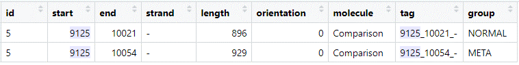
Both predictions have the same end position (note that this is on the reverse (-) strand), but differ for the start codon position.
Start codon position
- Think about what additional information we can use to figure out what the most likely start codon is.
We know that in order to replicate the virus has to hijack the hosts translation machinery and use that to syntheize proteins from its mRNAs. For the mRNA to be “detected” by the ribosome it has to bind the Ribosome Binding Site (RBS) - a sequence motif upstream of the start codon. This motif is not universally the same across the bacterial kingdom. For example, Escherichia coli utilizes the Shine-Dalgarno sequence (SD), whereas Prevotella bryantii relies on binding of ribosomal protein S1 to the unstructured 5’-UTR. Take some time to look at Figure 1 (and/or S5) of this paper to see what these motifs look like.
Now lets generate these motifs plots for both our meta and normal prodigal prediction. To do this we first have to extract all sequences upstream of the predicted start codons and then generate a sequence logo, for example using ggseqlogo. We already have the gene coordinate files, but we also need the contig sequence (bin_01.fasta) that we will read with bioseq. See this script on how to extract the upstream sequences and generate the sequence logos. It uses the data from the previous step (namely the default_genes and meta.genes dataframe) so you can paste it under the code from before.
Also again, think of changing the file path for bin_01.fasta when running the code.
Start codon position
- Compare the sequence logos to that in the paper above, could this tell you something about the host range of this phage?
Lets take a look at the upstream sequences of the “9125” gene:
META: `ACAAAAGTATGAACGTGGAGCACATAATA ATG`
NORM: `GTAATAAAACTAGATATAAAAACTAATATT ATG`
Why do you think each mode chose this specific start codon? (remember what characetersitcs were used and the difference between
metaand normal - see the wiki)Based on the logos, which one would you pick?
In case you have weird symbols again, find the plot here.
Key Points