Visualizing an annotated viral genome

Overview

Teaching: min
Exercises: 90 min

Objectives

• Use Python to draw a map of a viral genome

• Visualize gene overlap and direction

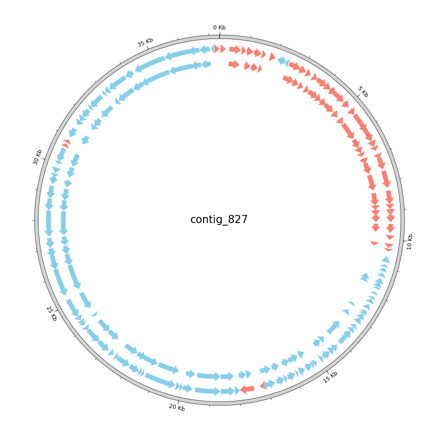
Next, we will visualize the differences in ORFs called by the two tools phannotate and prodigal-gv. Phannotate is used by Pharokka, which we ran to find genes and annotate them with funktions today. Yesterday we used CheckV to estimate the completeness of viral contigs. This tool is based on gene annotations found by prodigal-gv. To illustrate the difference between the two methods, we will plot the sets of genes used by both tools similar to the plots you generated today using Pharokka, which are based on the python package pyCirclize. The pyCirclize package provides tools to generate high-quality plots of annotated genomes in a circular layout, and allows for adding various data elements. Check the GitHub page to get an idea of its possibilities. To use the package, you have to install it into your virtual environment:

# activate the environment
$ source path/to/your/py3env/bin/activate

# install the packages we need
$ pip install pyCirclize

You can get some examples of how to use the package here. Starting from the first example, the Circos plot of the Enterobacter phage, adjust it to show both Phanotate and CheckV ORFs on your pet phage genome. We want to compare the differences in ORF calling. The information about the ORFs used by CheckV can be found in the tmp folder in your CheckV results (gene_features.tsv).

Exercise - plot two sets of gene predictions

Optional: Think about a way to convert the information in the TSV file into something parsable by pyCirclize and write a script for plotting the two sets of ORFs.

You can use the solution for the optional task above to create a .gff file from the gene predictions contained in the gene_features.tsv file of CheckV. If you run the script(s) on Draco, please remember to use slurm. The plotting script should not need much memory and can run on a single core.

Python script for converting tabular annotations into the GFF format

# This script expects three parameters to be passed to it. The path to CheckV's gene_features.tsv,
# the filename of the output .gff file and the name of the contig to be exported to gff.
 
import pandas as pd
import gffutils.gffwriter as gw
import gffutils.feature as gf
import os, sys

def main():

  # read parameters passed to the script. It ex
  in_file = os.path.abspath(sys.argv[1])
  assert in_file.endswith(".tsv")
	
  out_file = os.path.abspath(sys.argv[2])
  writer = gw.GFFWriter(out_file)
	
  contig_id = sys.argv[3]

  # read the .tsv file into a pandas dataframe (sep="\t" reads tab-separated files)
  df = pd.read_csv(in_file, sep="\t")
  # select the ORFs with the specified contig name
  df = df.loc[df["contig_id"] == contig_id]

  # iterate through the ORFs of the selcted contig
  for index, row in df.iterrows():
    # convert the strand integer into GFF-compatible "+" and "-"
    if row["strand"] == 1: strand = "+"
    else: strand = "-"
    # use gfutils to create a GFF feature from the information in the dataframe and append it to the output file 
    f = gf.Feature(seqid=row["contig_id"], featuretype="CDS", start=row["start"], end=row["end"], strand=strand)
    writer.write_rec(f)

  # close the writer to flush the writing buffer and properly finish the file
  writer.close()

if __name__ == "__main__":
    main()

python script for plotting ORFs with pyCirclize

# This script expects four paramerters passed to it. 1. The filename of the .gff file you generated with the above script,
# 2. the gff created by phannotate during todays practical session, 3. the filename of the output .png file and 4. the name
# of the contig you want to plot

from pycirclize import Circos
from pycirclize.parser import Gff
import os, sys

def main():
  # read the parameters passed to the script (see first comment for details)
  prodigal_filename = os.path.abspath(sys.argv[1])
  assert prodigal_filename.endswith(".gff")
	
  phanotate_filename = os.path.abspath(sys.argv[2])
  assert phanotate_filename.endswith(".gff")
	
  out_filename = os.path.abspath(sys.argv[3])
  assert out_filename.endswith(".png")
	
  contig_id = sys.argv[4]

  # use pycirclize's GFF parser to read the two input GFF files
  prodigal_gff = Gff(prodigal_filename)
  phanotate_gff = Gff(phanotate_filename)

  # Initialize circos sector by genome size
  circos = Circos(sectors={phanotate_gff.name: phanotate_gff.range_size})
  circos.text(contig_id, size=15)
  sector = circos.sectors[0]
	
  # Outer track: add size marks for the genome's length
  outer_track = sector.add_track((98, 100))
  outer_track.axis(fc="lightgrey")
  outer_track.xticks_by_interval(5000, label_formatter=lambda v: f"{v / 1000:.0f} Kb")
	outer_track.xticks_by_interval(1000, tick_length=1, show_label=False)
	
  # Plot forward & reverse CDS genomic features and color them differently for phannotate's ORF predictions
  cds_track = sector.add_track((90, 95))
  cds_track.genomic_features(phanotate_gff.extract_features("CDS", target_strand=1), plotstyle="arrow", fc="salmon")
  cds_track.genomic_features(phanotate_gff.extract_features("CDS", target_strand=-1), plotstyle="arrow", fc="skyblue")

  # Plot forward & reverse CDS genomic features and color them differently for prodigal's ORF predictions
  cds_track = sector.add_track((82, 87))
  cds_track.genomic_features(prodigal_gff.extract_features("CDS", target_strand=1), plotstyle="arrow", fc="salmon")
  cds_track.genomic_features(prodigal_gff.extract_features("CDS", target_strand=-1), plotstyle="arrow", fc="skyblue")

  # save plot to file
  circos.savefig(out_filename)
	
if __name__ == "__main__":
  main()

sbatch script for submitting the plotting script

#!/bin/bash
#SBATCH --tasks=1
#SBATCH --cpus-per-task=1
#SBATCH --partition=short
#SBATCH --mem=2G
#SBATCH --time=00:01:00
#SBATCH --job-name=plot
#SBATCH --output=./1.4_annotation/20_plot_viral_genome/viral_genome.slurm.%j.out
#SBATCH --error=./1.4_annotation/20_plot_viral_genome/viral_genome.slurm.%j.err

# activate the python virtual environment with the packages we need for plotting
source ./py3env/bin/activate

mkdir -p ./1.4_annotation/20_plot_viral_genome/

# define an array with contig ids to plot
declare -a arr=("contig_827" "contig_827")

features='./1.3_virus_identification/20_results_assessment_checkv/cross_assembly/tmp/gene_features.tsv'
outdir='./1.4_annotation/20_plot_viral_genome'
pharokka_dir='./1.4_annotation/10_pharokka/11_selected_contig'

# loop through the array
for contig in "${arr[@]}"
do
      echo $contig
      echo "$contig"
      # run the python script wich extracts the prodigal-gv-based annotations from the CheckV output
      # in this solution, the script expects three parameters:
      # first: the filname of the table generated by CheckV
      # second: the output filename for the filtered gff file
      # third: the contig id to filter for
      python python_scripts/annotation/10_table_to_gff.py $features $outdir/$contig.gff $contig
      
      # run the python script wich plots the two annotations in a circle
      # in this solution, the script expects four parameters:
      # first: the gff file of the prodigal-gv-based annotation created from CheckV's gene_features.gff
      # second: the gff file created by phanotate 
      # third: the output file name
      # fourth: the contig id to write into the plot

      python python_scripts/annotation/10_viral_genome.py $outdir/$contig.gff $pharokka_dir/$contig.gff $outdir/"$contig"_circos.png $contig
done

deactivate

Compare the annotations

Describe the differences between the two gene annotations based on the plots you created. Does the visualization confer these differences well?

Key Points

• The pyCirclize package provides tools for plotting genomic data, e.g., the set of genes, in a circular layout.