Course introduction
Overview
Teaching: 60 min
Exercises: 0 minObjectives
Understand course scope and evaluation criteria
Start and plan an effective lab book
login into Draco
Viromics
Metagenomics of viruses, often referred to as Viromics, is the study of viral communities in a sample or environment through the direct sequencing and analysis of their genetic material. This avoids the need to isolate or culture the viruses, preventing the bias associated with isolation, and allowing the complete viral community to be analyzed. This allows for the identification and characterization of both known and novel viruses within a given ecosystem. In this module, you will learn how to analyse viromics data with computational approaches.
Data
We will be using viromics sequencing data from Dr. Xiu Jia, a Postdoc in the VEO Group. This is data was generated by sequencing samples from the Unterwarnow, an estuary near Rostock. The samples were filtered through a 0.22um filter (commonly used to filter viral particles) and then sequenced on a Oxford Nanopore Technologies Flow Cell (long read sequencing).
Theory
The theoretical parts of the course are covered in the mornings. This includes reading relevant papers, watching video lectures, and discussion of the concepts and tools. Please write down any questions and discussion points about the theory in your Lab Notebook (see below).
Hands-on
The practical parts of the course are covered in the afternoons. You will use different bioinformatics tools, compare and interpret the results, and make conclusions about the sampled viruses. We will be available to help and guide you during this time. Please document how you performed the analyses, and write down any questions and discussion points in your Lab Notebook (see below). Solutions for each step are provided. If necessary, you can use them to move to the next steps.
Homework
For some of the tutorials, we will assign some homework (in lieu of the missed day on Friday 20 September). This is usually a visualization exercise. It will be up to you to complete this in your own time and to include it in your Lab Notebook and presentations.
Presentation
You will give a final presentation on Friday 27 September. This is where you can show off your understanding of the material and share what interesting things you have identified in the data.
Final evaluation
Your final grade is based on an evaluation of three factors.
- Your professional performance (active participation, asking questions, helping others): 30%
- Your Lab Notebook (approach to address hands-on questions/exercises, tidiness/reproducibility, notes/questions/discussion points): 30%
- The presentation of your final project: 40%
Lab Notebook
Documenting your work is crucial in Computational Biology/Bioinformatics. This way you can make sure your work is reproducible, document your commands to later find back what you did, prepare a first draft of text for other documents (e.g. a Methods section in a report or paper), and collect information which you can send to colleagues. Make sure that it is tidy, commented, and clearly written, so that others can easily understand it, including your future self.
You are required to write a Lab Notebook in markdown for this module, which will count as part of your evaluation. We recommend that you start a GitHub repository for the course and write your lab book there.
More details on your lab notebook
Access to Draco
Draco is a high-performance cluster created and maintained by the Universitätsrechenzentrum. It is available for members of Thuringian Universities. To log in, you can use ssh (replace <fsuid> by your FSU login):
ssh <fsuid>@login1.draco.uni-jena.de
Terminal or ssh client
More details on access to Draco
Submitting jobs on Draco
When you login to Draco, you are on the “login node” and this is not the best place to run any programs or heavier scripts. You MUST be on a “compute node” to run scripts and programs
You can either request for resources from a compute node and run programs interactively or submit a job to the job scheduler, which then sends it to a compute node to complete.
See here for what slurm architecture looks like
You can either request resources from a node for an “interactive” shell or you can submit via sbatch
To get resources - see here
To submit a job, you have to make a script my_slurm_script.sh and then submit it as sbatch my_slurm_script.sh . Detailed information on creating these scripts, including descriptions can be found in the “extras” here
Key Points
In this course, you will analyze viral sequence data
You need to keep a lab notebook
You need to be able to access the HPC Draco
Introduction to viromics
Overview
Teaching: 60 min
Exercises: 60 minObjectives
Summarize metagenomics and viromics
Understand what are bacteriophages and how they fit into microbial communities
Compare and contrast microbial and viral diversity
Video on viral metagenomics
Below is a lecture video introducing the concepts of metagenomics, microbial dark matter, and viromics. The case study covered in the video is about crAssphage, a type of bacteriophage that was first found using bioinformatics, by reanalyzing viromics data from the human gut by using the cross-assembly approach. The prevalence and implications of crAssphage are also discussed.
Exercise
Watch the lecture below and write down at least 3 questions and/or discussion points about it.
- Click on the image to see lecture video “Viral metagenomics: predicting phage-microbe interactions in the gut” by Prof Bas E. Dutilh (34 minutes):

Additional reading: Virus Bioinformatics (Pappas et al. 2021)
Exercise - mindmap
Create a mindmap summarizing the following points from the video. A mindmap is a brainstorming graphic. You can get creative using PowerPoint or draw it on paper, take a picture, and upload it into your Lab Notebook.
- What is metagenomics?
- What is viromics?
- What are bacteriophages and how prevalent and abundant are they?
- What are the roles of phages in microbial communities?
- more general, how do they influence the ecology and the environment
- Explain at least three ways that phages can have an impact on bacteria.
- More specifically, how do they influence their host (lytic/ temperate, HGT etc)
- Name at least three differences between the evolution of viral and cellular organisms?
Key Points
Viromics is the study of viruses, and in our case bacteriophages, using next-generation sequencing technologies
Bacteriophages are diverse and ubiquitous across all biomes
Bacteriophages have large implications on their environment including the human gut
Getting to know your files
Overview
Teaching: 120 min
Exercises: 0 minObjectives
Interpret different file formats used in bioinformatics
Utilize bash commands to look into sequence data
Get a basic understanding of what sequence data looks like
Work with sequence data in Python or R to create basic plots
Navigating your filesystem space
First, let’s copy the sequence data to your own home folders.
Exercise - get your sequence data
The data is in the folder
/work/groups/VEO/shared_data/Viromics2024Workspace/data/sequences/viral_metagenome# make a ./data/sequences directory if it doesn't already exist IN YOUR OWN HOME DIRECTORY mkdir -p viromics/data/sequences # go into your sequences directory cd viromics/data/sequences # copy over the 3 barcode files you need cp /work/groups/VEO/shared_data/Viromics2024Workspace/data/sequences/viral_metagenome/full_barcode*.fastq.gz ./
Exercise - check out your files
- Take a look at the file structure and files. We have given you a subset of viromics data
./data/sequences. Some helpful commands might be: Hint: for gzipped files - you need to zcat them first. e.g.zcat file.fastq.gz | head -10# list ls ll # path to working directory pwd # print first 10 lines zcat file.fastq.gz | head -10 # print last 10 lines zcat file.fastq.gz | tail -10 # open file on terminal (press 'q' to exit less) less more # count number of lines wc -l file.txt # search for "@" inside file grep "@" file.fastq # or gzipped files zgrep "@" file.fastq.gz | head -10 # count number of sequence headers in a fasta file grep -c ">" file.fasta zgrep -c ">" file.fasta.gz
See more useful commands and one-liners here
For creating new directories - please ensure to name your directories with a number and a meaningful header. An example is here
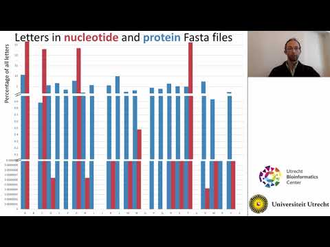
Understanding bioinformatics file formats
It is always a good idea to check the contents of your data files and make regular “sanity checks” to see if you understand everything. The first video covers different file formats commonly used in bioinformatics. Namely, FASTA, FASTQ, BAM, SAM, VCF, BCF, GFF, GTF and BED files (9 minutes).
The second video covers different types of sequence files, including fasta and fastq, phred scores, files containing metadata (tsv files) and compressed files (11 minutes).
Exercise
- What information is contained in sequencing files?
a) Choose 3 file formats and describe them- Choose the barcode62.fastq.gz file in your data/sequences/ folder
a) How many lines does this file have?
b) How many sequences are present in the file?- Print the first 5 lines and the last 5 lines in the terminal.
Hint: for gzipped files - you need to zcat them first. e.g.zcat file.fastq.gz | head -10
You don’t need to print this output into your lab-book
zcat barcode62.fastq.gz | cut -b -100 | head -10- to print the first 100 characters of the first 10 lines
a) What differences do you observe between these lines?
Key Points
Sequence data and information about genes and genomes can come in many different formats
The most common file formats are fasta (nucl. and amino acid), fastq, sam and bam, genbank, gff and tsv files
Sequencing Quality Control
Overview
Teaching: 180 min
Exercises: 0 minObjectives
Understand the value of sequencing quality control
Discuss how low quality reads affect genomic analysis
Perform quality check on long-read data by creating plots
Interpret quality check results
Perform quality control on reads
![]()
Every step of a metagenomics/viromics analysis pipeline needs quality control and sanity checks.
- What data am I working with?
- What is the quality of the data?
- Are my results what I expected them to be? Why?/Why not?
Here, we will assess the quality of DNA sequencing.
Sequencing quality control can include:
- Removing barcodes (i.e. oligonucleotides that were artificially added to identify sequences from a particular sample)
- Removing sequencing adapters (i.e. oligonucleotides that were artificially added to facilitate the sequencing process)
- Removing low-quality nucleotides (sequencing quality often drops towards the end of the reads)
- Filtering out reads based on quality scores (some reads are derived from faulty clusters or pores, and are best ignored)
Note that the Nanopore sequencing basecallers (Guppy/Dorado) already do quality control for us, but we will perform an extra check anyway.
Exercise
Discuss with your classmates and TAs:
- Why do we need quality control?
- What is the impact of including low-quality reads in downstream analyses?
- What are some metrics for assessing sequencing quality?
Assessing Sequencing Quality
We will use NanoPlot to assess the quality of our reads. NanoPlot is designed for long reads and uses information in the sequence files and also the metadata files to produce plots to evaluate the quality of our reads.
Exercise
- Run NanoPlot on your reads
- Assess the sequencing quality for each sample using default parameters
- Use fastq files and summary.txt located
./data/sequences/to generate diff types of quality plots (see the NanoPlot github)- Play around with the parameters such as colours and types of plots to generate
# to run nanoplot - you will need to source and activate the following conda environment:
source /vast/groups/VEO/tools/anaconda3/etc/profile.d/conda.sh && conda activate nanoplot_v1.41.3

NanoPlot -t ? --plots ? --color ? --fastq barcode1.fastq.gz -o output_dir/barcode1
Resources
Information about Nanopore sequencing quality and Phred scores
How to write a for-loop to loop through your files
sbatch script for NanoPlot
#!/bin/bash
#SBATCH --tasks=1
#SBATCH --cpus-per-task=10
#SBATCH --partition=short,standard,interactive
#SBATCH --mem=1G
#SBATCH --time=2:00:00
#SBATCH --job-name=sequencing_QC
#SBATCH --output=1.1_QC/10_nanoplot/nanoplot.slurm.out.%j
#SBATCH --error=1.1_QC/10_nanoplot/nanoplot.slurm.err.%j

# First, we check the quality of the reads using nanoplot
# activate the conda environment containing nanoplot

source /vast/groups/VEO/tools/anaconda3/etc/profile.d/conda.sh && conda activate nanoplot_v1.41.3

datadir="./data/sequences"
outdir="./1.1_QC/10_nanoplot"

# Run nanoplot on 3 fastq files in a for loop
# -t : threads (cpus)
# --plots : types of plots to produce, see gallery: https://gigabaseorgigabyte.wordpress.com/2017/06/01/example-gallery-of-nanoplot/
# --N50 : draw the N50 vertical line on the plots
# --color : color for the plots
# -o : output directory
# to see other options for colors and prefilters, run : NanoPlot -h

for fn in $datadir/full_barcode6*.fastq.gz
do
base_f=$(basename $fn .fastq.gz)        # select just the first part of the name
NanoPlot -t 10 --plots dot --N50 --color slateblue --fastq $fn -o $outdir/${base_f}/
done
This is an example of a plot you might get from NanoPlot. It is important to look at such a plot to estimate how much data will be lost when you filter by read quality or length.
- The top plot shows frequency of read lengths
- The large main plot shows how the read quality changes by read length
- The right plot shows the frequency of read qualities
Exercise
- How does the sequencing quality of the 3 samples compare to each other? Specify your answer with metrics from the NanoPlot results.
- Do we need to remove any reads? Why (not)?
- What does Q12 mean? How much data will be lost from each sample if we filter at Q12?
Filtering Reads
Many phages naturally have low-complexity regions in their genomes (e.g. ACACACACAC). Nanopore sequencing errors are biased towards low-complexity regions, either by falsely generating them or by exacerbating them. This can create artifacts in the assembled viral genome sequences. High-quality reads can significantly improve assemblies, particularly for error-prone long reads.
Exercise - filter your reads
- We will use Chopper to filter our reads based on quality scores and length. Build an sbatch script for chopper based on the following basic usage example. Use a for-loop that processes all your reads files. Use the following filtering criteria:
- minimum quality 14
- minimum length 1000 bp
- maximum length 40000 bp
# activate the conda environment
source /vast/groups/VEO/tools/anaconda3/etc/profile.d/conda.sh && conda activate chopper_v0.5.0
# base usage for filtering with minimum quality 10
gunzip -c reads.fastq.gz | chopper -q 10| gzip > filtered_reads.fastq.gz

# check the help for the other options
chopper -h
Chopper sbatch example
#!/bin/bash
#SBATCH --tasks=1
#SBATCH --cpus-per-task=10
#SBATCH --partition=short,standard
#SBATCH --mem=1G
#SBATCH --time=2:00:00
#SBATCH --job-name=sequencing_QC
#SBATCH --output=1.1_QC/20_chopper/chopper.slurm.out.%j
#SBATCH --error=1.1_QC/20_chopper/chopper.slurm.err.%j

# activate the conda environment containing chopper

source /vast/groups/VEO/tools/anaconda3/etc/profile.d/conda.sh && conda activate chopper_v0.5.0

datadir="./data/sequences"
outdir="1.1_QC/20_chopper"

# gunzip : unzip the reads
# -q : minimum read quality to keep
# -l : minimum read length to keep
# gzip: rezip the filtered reads

for fn in ./data/sequences/*.fastq.gz
do

base_f=$(basename $fn .fastq.gz)        # select just the first part of the name
gunzip -c $fn | chopper -q 14 -l 1000 --maxlength 40000 | gzip > $outdir/${base_f}_filtered_reads.fastq.gz

done
Exercise
- How many reads do you have left after filtering? What percentage of the original reads were filtered?
- What is the average quality? Is this before or after filtering?
- Optional: Run Nanoplot again to show the difference in the read statistics
GC Content
GC Content ((sum of all G’s + C’s) / (sum of all T’s + A’s)) is another interesting metric to evaluate your sequencing data. There’s no “wrong” GC content, rather this measure tells us something about the nucleic acid diversity our metagenomes/viromes. GC content is generally consistent along the length of a genome, as the GC content of sequencing reads from a single genome follows a bell curve. Regions with outlier values often represent non-self regions, for example a horizontally transferred gene, an inserted prophage, or a mobile genetic element. GC content is generally consistent for genomes of similar strains.
To compute and visualize the GC content of the reads, we will use python. We will need python throughout the course and make use of a virtual environment. Please setup a virtual environment according to this tutorial. The tutorial also shows you how to install any packages you might need for this analysis.
Exercise - GC content plots
Copy over the T4 phage genome
cp /work/groups/VEO/shared_data/Viromics2024Workspace/data/sequences/T4_SRR29341083.fastq.gz ./data/sequences
- What is the GC content profile of your sequenced reads?
a) Plot the distribution of GC % in each read as a density plot (histogram).
- Use the unfiltered reads
- install these useful Python packages:
- biopython
- numpy
- pandas
- matplotlib
Interpret the distributions:- Are these histograms what you expected?
- How would the GC content of a metagenome differ from these viromes?
- Describe the difference in GC content between our viromes and E. coli phage T4
/work/groups/VEO/shared_data/Viromics2024Workspace/data/sequences/T4_SRR29341083.fastq.gz).- What interpretations can you make about the samples based on these plots?
To make these GC_content plots, you will probably need the following python libraries and their functions:
- Bio.SeqUtils: gc_fraction
- Bio.SeqIO: parse
- pandas: DataFrame, transform
- numpy: arrange
- gzip
- sys
- matplotlib: hist
python script to make GC_content plots
To install the libraries
source ./py3env/bin/activate
pip install biopython, pandas, numpy, matplotlib
#! usr/bin/python3 # import libraries into your script from Bio.SeqUtils import gc_fraction from Bio import SeqIO import pandas as pd import numpy as np import gzip, sys import matplotlib.pyplot as plt fastq_dir=sys.argv[1] T4_path=sys.argv[2] # read in fastq.gz files gc_62={} with gzip.open(f"{fastq_dir}/full_barcode62_filtered_reads.fastq.gz", 'rt') as f: for record in SeqIO.parse(f, "fastq"): gc_62[record.id]=gc_fraction(record.seq)*100 print("gc_62... done") gc_63={} with gzip.open(f"{fastq_dir}/full_barcode62_filtered_reads.fastq.gz", 'rt') as f: for record in SeqIO.parse(f, "fastq"): gc_63[record.id]=gc_fraction(record.seq)*100 print("gc_63... done") gc_64={} with gzip.open(f"{fastq_dir}/full_barcode62_filtered_reads.fastq.gz", 'rt') as f: for record in SeqIO.parse(f, "fastq"): gc_64[record.id]=gc_fraction(record.seq)*100 print("gc_64... done") gc_T4={} with gzip.open(T4_path, 'rt') as f: for record in SeqIO.parse(f, "fastq"): gc_T4[record.id]=gc_fraction(record.seq)*100 #print(gc_fraction(record.seq)*100) print("gc_T4... done") # convert to a pandas dataframe # For your samples df_62 = pd.DataFrame([gc_62]) df_62 = df_62.T df_63 = pd.DataFrame([gc_63]) df_63 = df_63.T df_64 = pd.DataFrame([gc_64]) df_64 = df_64.T # For T4 phage df_T4 = pd.DataFrame([gc_T4]) df_T4 = df_T4.T # make a plotting function def make_plot(axs): # We can set the number of bins with the *bins* keyword argument. n_bins = 150 ax1 = axs[0] ax1.hist(df_62, bins=n_bins) ax1.set_title('% GC content') ax1.set_ylabel('Barcode 62') ax1.set_xlim(0, 100) ax1.set_xticks(np.arange(0, 100, step=10)) ax2 = axs[1] ax2.hist(df_63, bins=n_bins) ax2.set_ylabel('Barcode 63') ax3 = axs[2] ax3.hist(df_64, bins=n_bins) ax3.set_ylabel('Barcode 64') ax4 = axs[3] ax4.hist(df_T4, bins=n_bins) ax4.set_ylabel('T4 Phage') # Plot: fig, axs = plt.subplots(4,1, sharex=True, tight_layout=True) make_plot(axs) plt.show() # save your plot fig.savefig('GC_Content.png', dpi=150)
Run sbatch for gc plots
#!/bin/bash
#SBATCH --tasks=1
#SBATCH --cpus-per-task=1
#SBATCH --partition=short
#SBATCH --mem=1G
#SBATCH --time=00:30:00
#SBATCH --job-name=gc_plots
#SBATCH --output=1.1_QC/30_gc_plots/gc_plot.slurm.out.%j
#SBATCH --error=1.1_QC/30_gc_plots/gc_plot.slurm.err.%j

# activate the py3env
source ./py3env/bin/activate

# first argument: fastq files directory path
# second argument: T4 file path
python3 ./python_scripts/qc/gc_content.py ./1.1_QC/20_chopper ./data/sequences/T4_SRR29341083.fastq.gz

deactivate
Key Points
Sequencing quality control is an important first evaluation of our data
NanoPlot can be used to evaluate read quality of long reads
Chopper can be used to filter reads based on quality and/or length
The GC content profile of a metagenome or virome is composed of a mix of bell curves
Assembly lecture
Overview
Teaching: 60 min
Exercises: 30 minObjectives
Watch the lecture videos and read about assembly algorithms
![]()
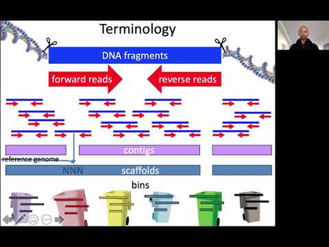
Sequence assembly is the reconstruction of long contiguous sequences (called contigs or scaffolds, see video below) from short sequencing reads. Before 2014, a common approach in metagenomics was to compare the short sequencing reads to the genomes of known organisms in the database (and some studies today still take this approach). However, this only works if the organisms in the database are closely related to the ones in the metagenomic sample. Recall that most of the sequences in a metavirome are unknown (“viral dark matter”), meaning that they yield no matches when compared to the reference database. Because of this, we need database-independent approaches to reconstruct new viral sequences. As sequencing technology and bioinformatic tools improved, sequence assembly enabled the recovery of longer sequences from metagenomic data. Having a longer sequence means having more information to classify it, so using metagenome assembly helps to characterize complex communities.
Video on sequence assembly
Watch the lecture video “Assembly strategies for genomics and metagenomics”. It will introduce reference-guided and de-novo assembly of genomic and metagenomic sequences (56 minutes):
Discussion
Watch the lecture video below and write down at least 3 questions and/or discussion points about it.
- Click on the image to see lecture video “Assembly strategies for genomics and metagenomics” by Prof Bas E. Dutilh (56 minutes):
Questions
- Would you use DBG (De-Bruijn Graph) or OLC (Overlap-Layout-Consensus) to assemble a dataset consisting of one billion short sequencing reads?
- What are the strengths and weaknesses of reference-guided assembly and de novo assembly?
- Would you use reference-guided or de novo assembly to assemble the genome of a model organism to discover mutations that occurred during an evolutionary experiment?
- Would you use reference-guided or de novo assembly to determine the genome sequence of an unknown organism?
- Why does metagenome assembly generally yield shorter contigs than genome assembly?
Additional reading: Computational Biology: Genomes, Networks, Evolution MIT course 6.047/6.878 (Prof. Manolis Kellis). This book is part of a course on Computational Biology and contains several topics that are relevant for Bioinformatics.
Read and summarize
Read the following sections and summarize shortly (less than half a page per section) their key points in your lab book:
- “5.2 Genome Assembly I: Overlap-Layout-Consensus Approach” and “5.3 Genome Assembly II: String graph methods” (pages 93 to 102).
Key Points
Sequence assembly can be used to assemble genomes from reads
Metagenome assembly generally yields shorter contigs than genome assembly
Assembly and cross-assembly
Overview
Teaching: 30 min
Exercises: 180 minObjectives
Assemble the metavirome from 3 samples
In this lesson, you will assemble the metavirome in two different ways using the tool Flye introduced in this article. Flye was designed to work well with noisy long reads and for metagenomic samples. Since you work on Draco, everything even slightly computationally expensive will be run through slurm. Please organize all the following steps in one or more sbatch scripts, as you learned yesterday. Since every tool needs different resources, it is recommended to have a single script per tool. All code snippets presented here assume that you put them in an adequate sbatch script. The necessary resources are mentioned in the comments or descriptions.
Cross-assembly
In a cross-assembly, reads from multiple samples are combined and assembled together. This allows for the discovery of shared sequence elements between the samples. If a virus (or other sequence element) is present in several samples, its sequencing reads from the different samples may be assembled together in one contig. Of course, whether this happens depends on how similar the sequence elements are, and on the stringency settings of the assembly algorithm. To figure out which contigs are present in which sample, we can map the sequencing reads from each sample to the contigs, and estimate the abundance by measuring the depth of coverage, i.e. the number of times that each nucleotide occurs in the reads. (We note that this can also be done with contigs that were assembled from a single metagenome.)
Exercise - Use flye to assemble a metagenome
You will perform a cross-assembly of the samples you started working with yesterday. To this end, you will first concatenate the sample files and then run Flye on the merged file. Gzipped files can be concatenated just like text files with the command line tool cat. Flye is installed in a conda environment on Draco.
# activate conda environment with flye installation on Draco
source /vast/groups/VEO/tools/miniconda3_2024/etc/profile.d/conda.sh && conda activate flye_v2.9.2

# merge the sequences
cat /path/to/*.fastq.gz > /path/to/all_samples.fastq.gz

# create a folder for the output cross-assembly
mkdir -p 10_results_assembly_flye/cross_assembly

# complete the flye command. This is the computationally expensive part
# and profits from many cores (30 is a good number). The used memory should
# not exceed 20GB of RAM. Think about the parameters you can pass to flye listed
# in the link below.
flye --nano-raw /path/to/all_samples.fastq.gz --meta --out-dir 10_results_assembly_flye/cross_assembly
Here you can find an overview over the possible parameters. Flye can be used for single-organism assemblies as well as metagenomic assemblies. Your sequences were generated with the Nanopore MinION platform and filtered to contain only high quality reads. You can pass an estimate of the size of your metagenome to flye, i.e., the combined length of the assembled contigs. It is difficult to accurately predict this if you do not know what’s in your samples (as in our case). How would you very roughly estimate this number?
After you have finalized your sbatch script with the resource assignments and the completed commands, you can either run it directly, or continue to expand it with the commands for the second approach described below. If you run it now, remember you can check the output of your script in the slurm log files which you can set with the sbatch parameters at the beginning of your script. Check both files. Often, the error output contains more than just errors, and this file is the more informative one.
#SBATCH --output=10_results_assembly_flye/assembly_flye.slurm.%j.out
#SBATCH --error=10_results_assembly_flye/assembly_flye.slurm.%j.err
Flye creates an assembly in multiple steps. You can read through the Flye log file that you defined with the
#SBATCH --error=parameter. Afterward, you can find a list of all assembled contigs with additional information in the fileassembly_info.txt, located in the Flye output folder.
- What are the longest and shortest contig lengths?
- What is the range of depth (coverage) values?
- How many circular contigs were assembled? Do you think this percentage is high or low?
- How does your guess about the size of the metagenome (above) compare to the actual size?
Separate assemblies
This part is recommended but optional. If you cannot finish it in the suggested time, move on to the next section “Assessing assembly quality”, which will be important for the coming days.
The second approach consists of performing separate assemblies for each sample and merging the resulting contigs by similarity in the end. Note that if a species is present in several samples, this final set will contain multiple contigs representing the same sequence, each coming from one sample. Because of this, we will further de-replicate the final contigs to get representative sequences.
Exercise - Use flye to assemble each sample individually
To run separate assemblies, you can adapt the flye command used for the cross-assembly to take each sample file individually and output the assemblies in separate folders in 10_results_assembly_flye. For this you can run a for loop over the respective files. The following expects the sample files to be called barcodeN.fastq.gz with N in (62, 63, 64):
# The individual assemblies need less memory than the cross-assembly,
# but you can still use the same resources as before.
for barcode in $(seq 62 64)
do
	flye ... /path/to/barcode$barcode.fastq.gz ...
done
Here, the command seq generates a sequence of integer numbers between its two arguments. Once the assemblies have finished, you will combine the contigs generated for each sample into a single file. Since the generated contigs are only assigned numbers by flye (not necessarily sequential), the same names will be present in each assembly. We have to rename them according to the sample they originate from for all contigs to have unique names. We can do this using Python and the Biopython package. Biopython provides many tools for the analysis of sequencing data, including tools for parsing and writing .fasta files. You can find the documentation on these here.
To use this Python package on Draco, use the virtual environment you set up yesterday. If you did not already install the
biopythonpackage yesterday, do so now. You can now write a python script that reads your contigs, changes their name, and writes a new file with the results using biopython. The basic structure of the script could look like this:from Bio import SeqIO import os, sys # read the arguments passed to your script. They are stored as a list in sys.argv. # sys.argv contains the parameters passed to the python binary, so sys.argv[0] # always contains the file name of your script. The arguments passed to the script # then start at sys.argv[1] assembly = os.path.abspath(sys.argv[1]) # open a file handle using the with open(x) as y syntax. This ensures the file is # closed properly after the code block. with open(assembly) as file_handle: for record in SeqIO.parse(file_handle, "fasta"): # do something with the sequence name # write the records with the new names ...This script should not be computationally expensive, but we will anyways execute it from within an sbatch script. We can also combine it with the script or scripts you already have written for the assemblies themselves. In this case, it is important to deactivate the conda environment holding the flye installation before activating the environment you just created.
python script for renaming contigs
import os, sys
from Bio import SeqIO

def main():

   # access parameters passed to your script
   assembly = os.path.abspath(sys.argv[1])

   # throw an error if the statement behind assert is not true
   assert assembly.endswith(".fasta")

   out_fasta = os.path.abspath(sys.argv[2])
   assert out_fasta.endswith(".fasta")

   sample_id = sys.argv[3]

   # modify names of the scaffols and store in to_write list
   to_write = list()
   with open(assembly) as handle:
       for record in SeqIO.parse(handle, "fasta"):
           # make sure not to do this twice, if run several times. Its not necessary.
           if record.id.startswith(sample_id): continue

           # adjust the id of the record object
           record.id = f"{sample_id}_{record.id}"

           # append the object to the list for writing back to a file later.
           to_write.append(record)

   # write records in to_write to .fasta file
   with open(out_fasta, "w") as fout:
       SeqIO.write(to_write, fout, "fasta")


if __name__ == "__main__":
   main()
sbatch script for assemblies
#!/bin/bash
#SBATCH --tasks=1
#SBATCH --cpus-per-task=32
#SBATCH --partition=short,standard,interactive
#SBATCH --mem=20G
#SBATCH --time=01:00:00
#SBATCH --job-name=assembly_flye
#SBATCH --output=./1.2_assembly/10_results_assembly_flye/assembly_flye.slurm.%j.out
#SBATCH --error=./1.2_assembly/10_results_assembly_flye/assembly_flye.slurm.%j.err

# run flye in metagenomic mode for de-novo assembly of viral contigs
# First, activate the conda environment which holds the flye installation on draco:


# First, activate the conda environment which holds the flye installation on draco:
source /vast/groups/VEO/tools/miniconda3_2024/etc/profile.d/conda.sh && conda activate flye_v2.9.2

# set a data directory holding your samples in .fastq.gz format
datadir="1.1_QC/20_chopper"

# create a merged fastq.gz file by concatenating three samples:
cat $datadir/barcode*_filtered_reads.fastq.gz > $datadir/merged_filtered.fastq.gz

# set a directory for ouputting results
outdir="./1.2_assembly/10_results_assembly_flye/cross_assembly"

# create a folder for the cross-assembly
mkdir -p $outdir

# flye parameters (https://gensoft.pasteur.fr/docs/Flye/2.9/USAGE.html)
# --nano-raw: tells flye about the input data. --nano-hq is also possible but results in a smaller assembly (Why?).
# --meta: for metagenomes with uneven coverage
# --genome-size: estimated size for metagenome assembly (mg size)
# -t: threads
flye --nano-raw $datadir/merged_filtered.fastq.gz --meta --genome-size 30m --out-dir $outdir -t 30

# single assemblies
# Run flye on all samples sequentially, save the results in separate folders named like the samples:

outdir="./1.2_assembly/10_results_assembly_flye/single_assemblies"
mkdir -p $outdir
for barcode in $(seq 62 64)
do
        flye --nano-raw $datadir/barcode${barcode}_filtered_reads.fastq.gz --meta --genome-size 10m --out-dir $outdir/barcode$barcode -t 30
done

# close the conda environment
conda deactivate

# activate your virtual environment
source ./py3env/bin/activate

# rename the contings in the generated single assemblies with a python script.
# It assumes three parameters here, first the input file name, second the output file name and third,
# the sample name to add to each contig name in the respective fasta file.
for barcode in $(seq 62 64)
do
        python3 python_scripts/assembly/10_run_rename_scaffolds.py $outdir/barcode$barcode/assembly.fasta $outdir/barcode$barcode.fasta barcode$barcode
done

deactivate

cat $outdir/barcode*.fasta > $outdir/assembly.fasta
Detecting similar sequences within and between assemblies
Some samples will contain the same virus strains. This will lead to the assembly of the same sequence in several times. To de-replicate the scaffolds of the single asseblies, we will cluster them at 95% Average Nucleotide Identify (ANI) over 85% of the length of the shorter sequence. These cutoffs are often used to cluster viral genomes at the species rank. This can be done with the tool vClust and results in both, clustering complete viral genomes at the species level and clustering genome fragments along with very similar and longer sequences.
Exercise - use vClust to find simililar contigs
vClust can also output cluster representatives, which will be the longest sequences within a cluster. Use this mode to get the information we need to dereplicate our merged single assemblies. Also apply vClust to the cross-assembly, this will give us more information on the assembled sequences. You can play with the similarity cutoffs (and metrics) used for clustering to see how they affect the results. vClust needs to align all sequences to each other and can run heavily in parallel. Remember to put this step into a sbatch script again and assign around 30 cores and 20GB of RAM.
# vClust is a python script and can be run by simply calling it on draco
# you have to run it with python 3.9
vclust='python3.9 /home/groups/VEO/tools/vclust/v1.0.3/vclust.py'

$vclust prefilter -i 10_results_assembly_flye/single_assemblies/assembly.fasta ...
$vclust align ...
$vclust cluster ...
After vClust ran successfully, you need to write a Python script to filter the assembly according to the information provided by vClust. To parse a tabular file in the format of CSV or TSV (comma- or tab-separated valus), the Python package pandas can be used. If its not in your virtual environment, install it now.
Now you can write a Python script that filters the assemblies corresponding to the output of vClust:
from Bio import SeqIO
import pandas as pd
import os, sys

# read the tsv file generated by vClust
cluster_df = pd.read_csv('path/to/the/file.tsv', sep='\t')

with open(assembly) as file_handle:
  for record in SeqIO.parse(file_handle, "fasta"):
    # check if the contig is in the set of representatives

# write the records which passed the test
...
Python script for filtering similar contigs
import os, sys
import pandas as pd
from Bio import SeqIO

def main():

    assembly_filename = os.path.abspath(sys.argv[1])
    assert assembly_filename.endswith(".fasta")

    out_filename = os.path.abspath(sys.argv[2])
    assert out_filename.endswith(".fasta")

    cluster_reps_filename = os.path.abspath(sys.argv[3])
    assert cluster_reps_filename.endswith(".tsv")

    cluster_reps_df = pd.read_csv(cluster_reps_filename, sep='\t')
    cluster_reps_set = set(cluster_reps_df["cluster"])

    to_write = list()
    with open(assembly_filename) as handle:
        for record in SeqIO.parse(handle, "fasta"):
            if record.id in cluster_reps_set: to_write.append(record)

    # write records in to_write to .fasta file
    with open(out_filename, "w") as fout:
        SeqIO.write(to_write, fout, "fasta")


if __name__ == "__main__":
    main()
sbatch script for dereplication
#!/bin/bash
#SBATCH --tasks=1
#SBATCH --cpus-per-task=32
#SBATCH --partition=short,standard,interactive
#SBATCH --mem=2G
#SBATCH --time=01:00:00
#SBATCH --job-name=assessment_vclust
#SBATCH --output=./1.2_assembly/20_results_assessment_vclust/assessment_vclust.slurm.%j.out
#SBATCH --error=./1.2_assembly/20_results_assessment_vclust/assessment_vclust.slurm.%j.err


vclust='python3.9 /home/groups/VEO/tools/vclust/v1.0.3/vclust.py'

indir='./1.2_assembly/10_results_assembly_flye/cross_assembly'
outdir='./1.2_assembly/20_results_assessment_vclust/cross_assembly'
mkdir -p $outdir

$vclust prefilter -i $indir/assembly.fasta -o $outdir/fltr.txt
$vclust align -i $indir/assembly.fasta -o $outdir/ani.tsv -t 30 --filter $outdir/fltr.txt
$vclust cluster -i $outdir/ani.tsv -o $outdir/clusters_tani_90.tsv --ids $outdir/ani.ids.tsv --metric tani --tani 0.90
$vclust cluster -i $outdir/ani.tsv -o $outdir/clusters_tani_70.tsv --ids $outdir/ani.ids.tsv --metric tani --tani 0.70
$vclust cluster -i $outdir/ani.tsv -o $outdir/clusters_ani_90.tsv --ids $outdir/ani.ids.tsv --metric ani --ani 0.90
$vclust cluster -i $outdir/ani.tsv -o $outdir/clusterreps.tsv --ids $outdir/ani.ids.tsv --algorithm uclust --metric ani --ani 0.95 --cov 0.85 --out-repr

source ./py3env/bin/activate

python3 ./python_scripts/assembly/20_run_filter_representatives.py $indir/assembly.fasta $outdir/assembly.fasta $outdir/clusterreps.tsv

deactivate

echo Done running python script for cross-assembly...

indir='./1.2_assembly/10_results_assembly_flye/single_assemblies'
outdir='./1.2_assembly/20_results_assessment_vclust/single_assemblies'
mkdir -p $outdir

$vclust prefilter -i $indir/assembly.fasta -o $outdir/fltr.txt
$vclust align -i $indir/assembly.fasta -o $outdir/ani.tsv -t 30 --filter $outdir/fltr.txt
$vclust cluster -i $outdir/ani.tsv -o $outdir/clusters_tani_90.tsv --ids $outdir/ani.ids.tsv --metric tani --tani 0.90
$vclust cluster -i $outdir/ani.tsv -o $outdir/clusters_tani_70.tsv --ids $outdir/ani.ids.tsv --metric tani --tani 0.70
$vclust cluster -i $outdir/ani.tsv -o $outdir/clusters_ani_90.tsv --ids $outdir/ani.ids.tsv --metric ani --ani 0.90
$vclust cluster -i $outdir/ani.tsv -o $outdir/clusterreps.tsv --ids $outdir/ani.ids.tsv --algorithm uclust --metric ani --ani 0.95 --cov 0.85 --out-repr

source ./py3env/bin/activate

python3 ./python_scripts/assembly/20_run_filter_representatives.py $indir/assembly.fasta $outdir/assembly.fasta $outdir/clusterreps.tsv

deactivate
Questions - Go through the results of vClust
vClust is a great tool to get a feeling for the diversity within your assemblies (or any kind of set of sequences).
- How many similar sequences were found in each assembly?
- How do the results depend on the choice of your metric (ANI, TANI, or GANI) and your cutoff values?
Key Points
Flye can be used to assemble long and noisy nanopore reads from metagenomic samples.
Samples can be assembled individually and combined in a cross-assembly
vClust can be used to assess the diversity of sequences in your assembly
Assessing assembly quality
Overview
Teaching: 0 min
Exercises: 120 minObjectives
Assess the quality of your assemblies
Now we will measure some basic aspects of the assemblies, such as the fragmentation degree and the percentage of the raw data they represent. A metagenome consists of all the genomic information of all the organisms in a given system. So in the ideal case, a metagenomic assembly would contain a single and complete contig for each chromosome or plasmid in the sample, in which case all the metagenomic sequencing reads can be perfectly mapped back to the assembly. Of course, this will never happen, because in most biomes there is a long tail of rare organisms that contribute only a tiny fraction of the sequenced DNA, so complete horizontal coverage of their genome cannot be achieved, and their assembly remains fragmented. Other problems are repeated regions in the metagenome and microdiversity between strains, which both lead to complex structures in the assembly graph, and thus fragmented assemblies.
Contig length distribution
To get a first idea about your assembly, it is helpful to look at the distribution of the length of the generated contigs. We can discribe this distribution using some numbers derived from it, such as the maximum, the median and something called N50 or N90. These numbers are computed by concatenating all contings ordered by their length. The length of the contig sitting at 50% (or 90%) of the total length of all contigs combined this way, is called N50 (or N90). The QUAST program (Gurevich et al., 2013) can be used to compute these values and visualize the distribution of the contig lengths. The tool can additionally use a reference sequence to compare the assembly against for assessing its fragmentation. We do not have a reference and will use the basic analysis of Quast.
Exercise - Use Quast to compute the contig length distribution
Use the Quast program to visualize the distribution of the contig lengths. You will need to run it two times, once per assembly, and save the results to different folders (ie.
result_quast/cross_assemblyandresult_quast/single_assemblies). Quast does not need many ressources. Assigning 2 CPUs and 5 GB of RAM for sbatch should be enough.# create a folder for the assessment within todays folder $ mkdir 30_results_assessment_quast # Quast is already installed on the server. Its a python script located here: $ quast='python3 /home/groups/VEO/tools/quast/v5.2.0/quast.py' # run quast two times, once per assembly $ $quast -o 30_results_assessment_quast/cross_assembly /path/to/your/cross_assembly/assembly.fasta # run quast again on the assembly.fasta, which is merged from your vclust results (merged x3 single assemblies) $ $quast -o 30_results_assessment_quast/single_assemblies ./1.2_assembly/20_results_assessment_vclust/single_assemblies/assembly.fastaYou can get the results from the file
report.txtor copy the whole results folder to your computer and openreport.htmlin your local browser.
sbatch script for running Quast
#!/bin/bash
#SBATCH --tasks=1
#SBATCH --cpus-per-task=2
#SBATCH --partition=short,standard,interactive
#SBATCH --mem=1G
#SBATCH --time=00:30:00
#SBATCH --job-name=assessment_quast
#SBATCH --output=./1.2_assembly/30_results_assessment_quast/assessment_quast.slurm.%j.out
#SBATCH --error=./1.2_assembly/30_results_assessment_quast/assessment_quast.slurm.%j.err

# Set some variables for the quast script on draco and the files to be analysed
quast='python3 /home/groups/VEO/tools/quast/v5.2.0/quast.py'
cross_assembly='./1.2_assembly/10_results_assembly_flye/cross_assembly/assembly.fasta'
single_assembly='./1.2_assembly/20_results_assessment_vclust/single_assemblies/assembly.fasta'
outdir='./1.2_assembly/30_results_assessment_quast'

# run Quast to visualize the distribution of contig lengths
$quast -o $outdir/cross_assembly $cross_assembly
$quast -o $outdir/single_assemblies $single_assembly
How well does the assembly represent the reads?
Next, we will test how much of the raw data (reads) is represented by the assembly
(contigs). We will use minimap2 to align the reads from each sample to the assembled
contigs and samtools to handle the output of minimap2.
Exercise - Map the reads back to the assembly with minimap2
You will map the reads from each barcode separately. Minimap2 is an alignment tool that outputs Sequence Alignment Map (SAM) file format, which has to be converted to a compressed binary (BAM) format and then sorted using
samtools viewandsamtools sort. You can also usesamtools sortto create index files, which facilitate quick access to the data in the binary file. Last, you can get basic stats of the mapping usingsamtools stats. This will tell you how many of the reads aligned to each of the assemblies, and how many did not align. You can also pipe the respective outputs of each step into the next step, saving disk IO and possibly speeding up things (minimap2 and samtools are specifically designed for this). You can read the manuals for minimap2 and samtools to figure out the specific commands to use (use the solution, if you’re short on time).# minimap2 and samtools are installed on draco and you can set aliases to their location: minimap2='/home/groups/VEO/tools/minimap2/v2.26/minimap2' samtools='/home/groups/VEO/tools/samtools/v1.17/bin/samtools' # pipe the commands into eachother. The '-' # tells the tools to take their input from the pipe: $ $minimap2 ... | $samtools view ... - | $samtools sort ... - # get mapping statistics of each bam file $ $samtools stats ...
samtools statscreates a long report with tabular statistics which could be plotted. The size of the output is determined by the maximum length of all reads and can get very large for alignments of long reads. A summary of the statistics is located at the beginning of the file and you can read the relevant first 46 lines with “head -46 path/to/stats/file.txt” or using “less path/to/stats/file.txt”. There is a lot of information contained in these lines, an important measure for us is the number of reads which could be mapped back to the assembly and also the number of bases mapped.
sbatch script for aligning the samples to the assemblies
#!/bin/bash
#SBATCH --tasks=1
#SBATCH --cpus-per-task=32
#SBATCH --partition=short,standard,interactive
#SBATCH --mem=2G
#SBATCH --time=00:30:00
#SBATCH --job-name=alignment_minimap2
#SBATCH --output=./1.2_assembly/40_results_alignment_minimap2/alignment_minimap2.slurm.%j.out
#SBATCH --error=./1.2_assembly/40_results_alignment_minimap2/alignment_minimap2.slurm.%j.err


# assign tool paths to aliases for better readability
minimap2='/home/groups/VEO/tools/minimap2/v2.26/minimap2'
samtools='/home/groups/VEO/tools/samtools/v1.17/bin/samtools'

# run minimap2 to align all reads from a sample to the assembled contigs
# and pipe the output into samtools for conversion into the binary bam format
#
# minimap2 parameters (https://lh3.github.io/minimap2/minimap2.html):
# -x map_ont : Use a preset for parameterizing the affine gap penalty model for the extension of matched seeds
# suited for noisy nanopore reads.
# -a : output in SAM format
# -t 30 : run with 30 threads
#
# samtools parameters (http://www.htslib.org/doc/samtools.html):
#
# samtools view can be used to convert between SAM, BAM and CRAM formats.
# view -u : output uncompressed binary format (BAM)
#
# samtools sort can be used to sort a SAM, BAM or CRAM file. Some tools expect sorted alignments.
# sort --write-index : output the index of the sorted alignments, can reduce file IO when accessing only a subset of the alignments
# sort -o : set the output file for the sorted alignments
#
# - : the - tells samtools to take the inpute from the pipe (| is the piping operator).


indir='./1.1_QC/20_chopper'

# cross-assembly
outdir='./data/alignments/cross_assembly'
assembly='./1.2_assembly/10_results_assembly_flye/cross_assembly/assembly.fasta'
mkdir -p $outdir

# loop through the numbers 62 to 64 and use it to generate diffenrent filenames within the loop
for barcode in $(seq 62 64)
do
 $minimap2 -x map-ont -a -t 30  $assembly $indir/barcode${barcode}_filtered_reads.fastq.gz | \
   $samtools view -u - | $samtools sort -o $outdir/barcode$barcode.bam --write-index -
 $samtools stats $outdir/barcode$barcode.bam > $outdir/barcode$barcode_stats.txt
done

# single assemblies
outdir='./data/alignments/single_assemblies'
assembly='./1.2_assembly/20_results_assessment_vclust/single_assemblies/assembly.fasta'
mkdir -p $outdir

for barcode in $(seq 62 64)
do
 $minimap2 -x map-ont -a -t 30 $assembly $indir/barcode${barcode}_filtered_reads.fastq.gz | \
   $samtools view -u - | $samtools sort -o $outdir/barcode$barcode.bam --write-index -
 $samtools stats $outdir/barcode$barcode.bam > $outdir/barcode$barcode_stats.txt
done
Questions - Compare both assemblies
You now have access to several metrics about your assemblies.
- The assembly data from Flye;
- The similarity between your contigs from vClust;
- N50, N90 and the distribution of contig lengths from Quast;
- The alignment of your reads to the assembled contigs from Minimap2/Samtools.
Can you summarize these results in a clear way and explain the difference between the assemblies? Focus on the difference between the cross-assembly and the separate assemblies.
- Which assembly has more contigs? Why?
- Which assembly has more contigs above a fixed length? Why?
- Which assembly better represents its input reads? Why?
- Can you think of other metrics to assess the quality of a metagenomic assembly?
Key Points
checkV assesses the quality of your contigs with regard to viral completeness and contamination
minimap2 aligns long and noisy nanopore reads efficiently to large (meta)genomes
samtools can be used to read, filter, convert and summarize alignments
Visualizing the assembly
Overview
Teaching: 0 min
Exercises: 90 minObjectives
Understand the topology of the de-Bruijn graph
Understand how the presence of similar species in the sample affects the assembly
This section is suggested as homework.
Choose one of the following two topics: “A. Paths in the de-Bruijn graph” or “B. Effect of related species”. Pick what sounds more interesting to you, and discuss your results with someone who picked the other topic. (Bandage is difficult to run on Windows.)
A. Paths in the de-Bruijn graph
We will use Bandage, a tool to visualize
the assembly graph. Bandage is difficult to run on a Windows computer. In the
releases section,
follow the instructions to download the most appropriate version, such as
Bandage_Ubuntu-x86-64_v0.9.0_AppImage.zip. To run it, unzip the file and
call Bandage from the terminal like this:
# run Bandage
$ ./Bandage_Ubuntu-x86-64_v0.9.0.AppImage
In File > Load_graph, navigate to and load the file assembly_graph.fastg of
the cross-assembly. Then click Draw graph to visualize the graph. Note that
this graph has already been compacted by collapsing nodes that form linear,
unbranching paths into unitigs. Nodes in the graph are called edge_N (confusing name…)
with N being an integer. They often correspond to the final contigs in your assembly.
Bubbles and junctions
Open the file
assembly_info.txtcorresponding to the graph you are looking at. The N in the node names as displayed by Bandage corresponds to the number assigned to continuous paths in the de-Bruijn graph by Flye. The “graph_path” column holds this information for all contigs.
- What does an asterisk * mean?
- What do multiple occurrences of the same number mean?
Pick two components of the visualized de-Bruijn graph and explain their topology and information content.
- Are there bubbles and junctions?
- Can you relate the complexity of the visualized graph to the Flye command line parameters?
B. Effect of related species
Metagenomic samples often contain several strains for a given species. This is particularly evident with viruses that typically contain many haplotypes. Each small difference between the genomes leads to a fork and a structure in the assembly graph. This complicates the path-finding algorithm implemented in the assembly tool. Mistakes at this point can lead to chimeric contigs containing sequences from more than one strain. To visualize this effect, we will align the reads in our samples back to the assembled contigs and use jbrowse2 to visualize the differences between reads and contigs. Download the tool. Under Linux or Mac, you can start the AppImage simply by typing
# run JBrowse2
$ ./jbrowse-desktop-v2.13.1-linux.AppImage
from within the corresponding folder. After starting JBrowse2, select
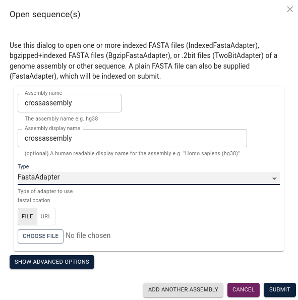
open sequence file(s):
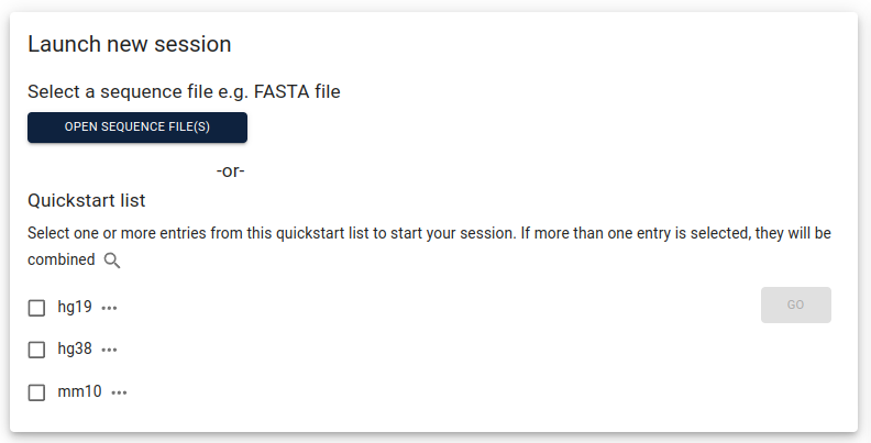
Assign a name to your assembly, select FastaAdapter under
Type and then choose file to navigate to your assembly file and submit:
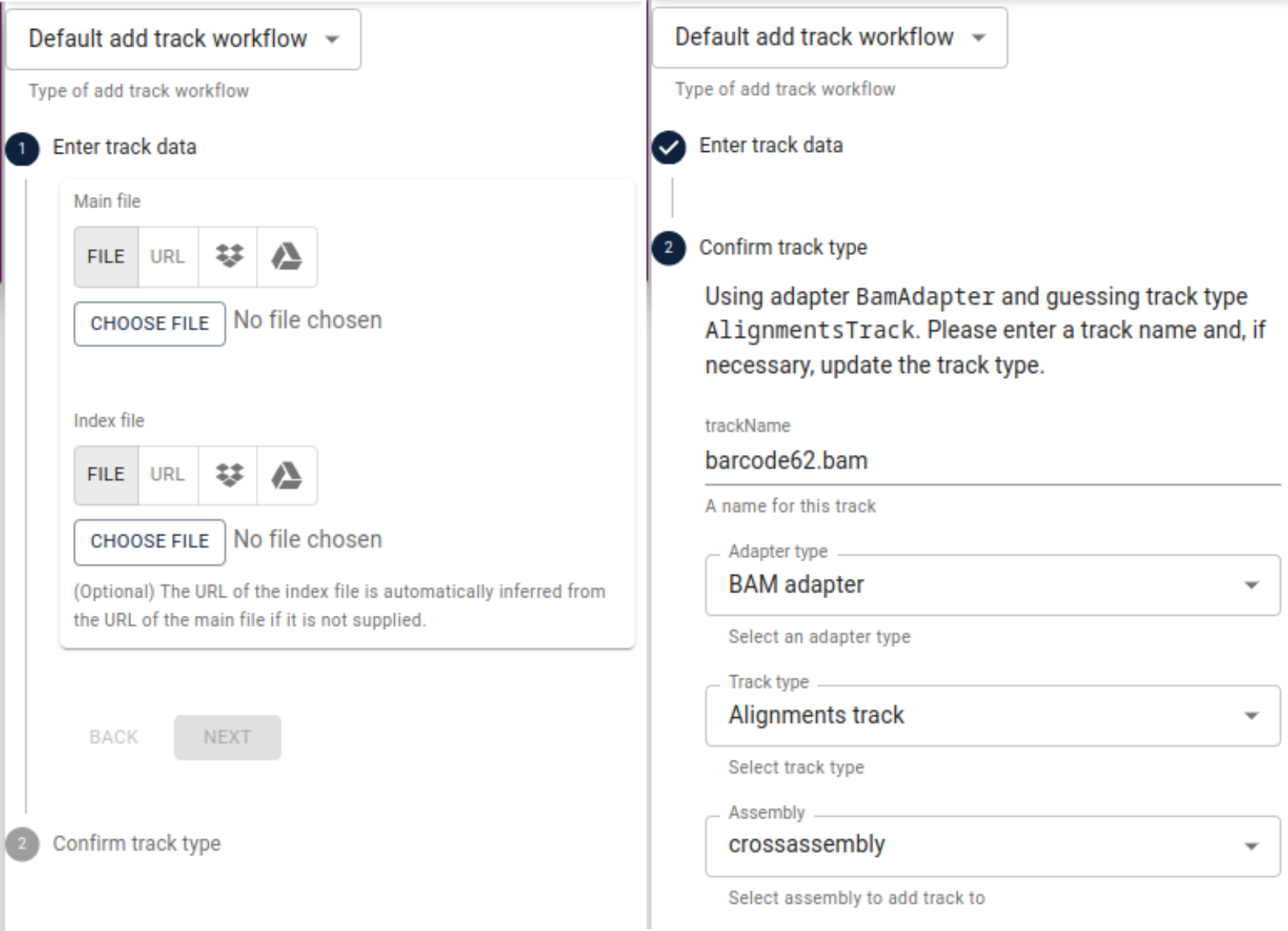
Click launch view with linear genome view selected, then show all regions in assembly
and “open track selector”, click the plus sign in the lower right corner and select
add track. Under main file, select File and then choose file and navigate to
the alignments you computed for the first of our three samples (e.g., “barcode62.bam”).
After that, repeat the same under index file and navigate to the index file of the
alignments (e.g., “barcode62.bam.csi”). Click Next and make sure, the IndexedBamAdapter
is selected and confirm.
Repeat this process for the other two alignment files and their adapter files. Now, you can inspect single reads aligned to your assembly. Try to familiarize yourself with the interface. You can search for a specific contig by typing its name into the search bar at the top of the interface.
Chimeras and reads connecting contigs
Try to look into contigs with a high coverage and find some wich have reads mapped to them in all three samples.
- Can you identify multiple virus strains visually? Make a screenshot, explain what you see, and how this fits into what you learned about assemblies with de-Bruijn graphs.
When clicking on an alignment, you can find alternative alignments of the same read to other contigs.
- Name at least one reason that (part of) a read could be aligned to multiple locations.
Key Points
Bandage can visualize the de-Bruijn graph
JBrowse2 can visualize genomic data like alignments and coverage
Identifying Viral Contigs I
Overview
Teaching: 0 min
Exercises: 180 minObjectives
Understand the concept and structure of benchmarking virus identification tools
Evaluate the benchmarking results presented in the paper by Wu et al
Choose a virus identification tool
![]()
Comparing Virus Identification Tools
In this theoretical part, you will dive into a very important part of microbiome data analysis: how to choose a good tool. Several tools have been developed over the past years for identifying viral sequences. Each tool measures different aspects of the sequence, applies different algorithms to extract and compare the information, and uses different reference databases to distinguish viral from non-viral sequences.
To choose the best one for your project, you should consider the overall performance of the tools (e.g. sensitivity and specificity, but also ask whether the purpose of the tool aligns with your research goal. If a recent tool does the same task as a previously published one, the authors should compare (or benchmark) them in their publication. But benchmarks can be biased, so ideally, bioinformatic tools are benchmarked by independent scientists.
Today, we will study the paper: “Benchmarking bioinformatic virus identification tools using real‐world metagenomic data across biomes” (Wu et al., 2024). Considering the allocated time for this activity, you will probably not be able to read the entire paper. To answer the proposed questions, please focus on Figures 1, 3, and 6 (and associated Methods and Results paragraphs, search online when necessary).
Questions
The authors investigated nine tools, which can be divided into three categories. What categories? Describe the basic approach of each category of tools.
What is meant by the sets of True Positives, False Negatives, False Positives, and True Negatives in Figure 1? Explain what each of these sets can tell us in the benchmark, and explain how they were generated.
In Figure 3 A/B/C, what indicates a good performance?
In Figure 3 D/E/F, the terms TPR, FPR, and AUC/ROC are used for evaluation. What are those terms? What is the main takeaway from these figures?
Overall, which types of tools perform better? Why do you think that is?
Explain what is shown in Figure 6. Do you believe it? What value does this analysis add to the benchmarking?
Considering all you have learned from the paper, is there an ideal tool to identify viral sequences? Why (not)?
For the project we are developing in this module, which tool(s) would you use? Why?
Key Points
Different approaches can be used in a virus identification tool, such as reference-based and machine learning
Benchmark is a comparison between tools and should offer concrete evidence of performance, such as number of TP, FN, FP and TN
When choosing a tool, you should consider the priorities of the project. E. g. you need to identify as many viruses as possible and FP are not critical, so a tool with high recall is ideal
Identifying viral contigs II
Overview
Teaching: 0 min
Exercises: 180 minObjectives
Select medium-complete and low-contaminated contigs
Identify phage contigs in assembled viromes and metagenomes
Interpret Jaeger’s output
Select viral contigs for further analysis
Assess assembly completeness
Understand differences between viromes and metagenomes
In this section, we will identify viral sequences among our assembled contigs. This morning, you studied how Wu et al. benchmarked nine bioinformatic virus identification tools. As many of those tools are quite slow, we will use a different tool that was developed by the VEO-MGX Groups: Jaeger. Jaeger was developed after the Wu et al. benchmarking study, so we will test how well it performs ourselves by running it on the cross-assembled virome contig dataset, and also on contigs from total community metagenomes from the same Unterwarnow estuary samples. We will compare the percentage of detected contigs to the numbers reported in the Wu et al. paper.
Document your activities and answer the questions below in your lab book. Do not forget to cite all relevant sources in your work.
Identify viral contigs
We will start to identify viral contigs with Jaeger.
Challenge
Viromes and metagenomes are obtained in the wet lab through different filtration steps. Smaller filters remove larger particles such as eukaryotes and prokaryotes. Where do you expect the most hits from Jaeger (virome or metagenome) and why?
Why is it important to use tools like Jaeger on viromes?
Note that Jaeger should require a bit more than 1 GB for the sbatch job, so make sure to allocate at least 2 GB of memory. Jaeger can run on CPU nodes, but it’s speed is optimal when run on GPU nodes. In the parameter --partition of the sbatch script, you could add gpu,short to allocate the job to a GPU node.
Exercise
Run Jaeger for cross-assembly:
- Read and interpret the output following Jaeger’s webpage
module load nvidia/cuda/12.1.0
source /vast/groups/VEO/tools/miniconda3_2024/etc/profile.d/conda.sh
conda activate jaeger_dev
python3 /home/groups/VEO/tools/jaeger/v1.1.30a0/Jaeger/bin/jaeger run -i <file> -o <output_file>
Inspect the output files After running Jaeger, answer the questions below.
head <output>
sbatch script for jaeger
>#!/bin/bash
#SBATCH --tasks=1
#SBATCH --cpus-per-task=10
#SBATCH --partition=standard
#SBATCH --mem=5G
#SBATCH --time=2:00:00
#SBATCH --job-name=jaeger
#SBATCH --output=./1.3_virus_identification/10_jaeger/jaeger.slurm.out.%j
#SBATCH --error=./1.3_virus_identification/10_jaeger/jaeger.slurm.err.%j

#The most updated version of Jaeger is from 20240806

module load nvidia/cuda/12.1.0
source /vast/groups/VEO/tools/miniconda3_2024/etc/profile.d/conda.sh
conda activate jaeger_dev

# from here on, we will just use the cross-assembly for our analyses

assembly='./1.2_assembly/10_results_assembly_flye/cross_assembly/assembly.fasta'
outdir='./1.3_virus_identification/10_jaeger'
jaeger='python3 /home/groups/VEO/tools/jaeger/v1.1.30a0/Jaeger/bin/jaeger run'

mkdir -p $outdir

$jaeger -i $assembly -o $outdir/results_jaeger
Questions
- Do the results corroborate your expectations?
- Why are not all contigs in the virome identified as viral contigs?
- Take the longest contig from the dataset and BLAST it using blastn. What are the top hits? Are they expected?
Optional: How many viral contigs are there in the virome?
bash command for getting the number of phage contigs
cut -f 3 <file> | sort | uniq -c
To get a command to get the sequence of a contigID, you coul go to “Extract contig fasta” of the tutorial of Gene Calling and Functional Annotation II.
Estimating genome completeness
There are tools to assess the completeness of bacterial and viral genome sequences. For viruses we use CheckV. The tool identifies genes on the query sequence and compares them to a database of viral and bacterial marker genes. Each taxonomic group of bacteria or phages, e.g. a species or a family, has certain marker genes on its genome. So based on the number and types of marker genes, CheckV can figure out to which taxon a query contig belongs and estimate how much of the genome it represents (estimated completeness). (We will improve the taxonomic annotation in the “Viral Taxonomy and Phylogeny” section next week.) CheckV also checks for unexpected marker genes on the sequence (estimated contamination), and whether part of a phage contig likely represents bacterial sequence, in which case the fragment could be part of a host genome with an integrated prophage.
# create a folder for the assessment (or let sbatch create it when you assign the output and error log files)
$ mkdir 30_results_assessment_checkv

# activate the conda environment containing the checkv installation
$ source /vast/groups/VEO/tools/anaconda3/etc/profile.d/conda.sh && conda activate checkv_v1.0.1

# run checkV on both assemblies
$ checkv end_to_end ...
sbatch script for running checkV
#!/bin/bash
#SBATCH --tasks=1
#SBATCH --cpus-per-task=22
#SBATCH --partition=standard
#SBATCH --mem=20G
#SBATCH --time=02:30:00
#SBATCH --job-name=assessment_checkv
#SBATCH --output=./1.3_virus_identification/20_results_assessment_checkv/assessment_checkv.slurm.%j.out
#SBATCH --error=./1.3_virus_identification/20_results_assessment_checkv/assessment_checkv.slurm.%j.err

# run CheckV to assess the completeness of single-contig virus genomes.
# First, activate the conda environment which holds the CheckV installation on draco:
source /vast/groups/VEO/tools/anaconda3/etc/profile.d/conda.sh && conda activate checkv_v1.0.1

# CheckV parameters (https://bitbucket.org/berkeleylab/checkv/src/master/#markdown-header-running-checkv)
# checkv end-to-end runs the CheckV pipeline from end to end :). It expects an input fasta file
# with the assembly and an output path.
# -t: threads

# assigning variables for readability

database='/work/groups/VEO/databases/checkv/v1.5'
outdir='./1.3_virus_identification/20_results_assessment_checkv'
cross_assembly='./1.2_assembly/10_results_assembly_flye/cross_assembly/assembly.fasta'
single_assembly='./1.2_assembly/20_results_assessment_vclust/single_assemblies/assembly.fasta'

checkv end_to_end -t 20 -d $database $cross_assembly $outdir/cross_assembly
checkv end_to_end -t 20 -d $database $single_assembly $outdir/single_assemblies
Go through the CheckV results
CheckV produces many output files, and also saves files for the intermediate steps of the tools that are used to find viral marker genes (diamond and hmmsearch). A summary of all results can be found in the file
quality_summary.tsv. Open the file and familiarize yourself with the information presented in the table. On CheckV’s website, you can find information about the output in the sections “How it works” and “Output files”.
- How are completeness and length related? (qualitative answer, name examples)
- What are reasons for contigs with low completeness to appear in the assembly?
- How do completeness and contig coverage relate? (qualitative answer, name examples)
Filter contigs
Exercise - select high-quality phage contigs
Use Jaeger’s predictions (‘phage’ and ‘non-phage’) and CheckV’s estimates of completeness and contamination to separate phage from non-phage contigs and reduce our assembly to high-quality contigs of high completeness. If you are an experienced programmer, write (a) script(s) for that. If you are not, use the solutions below. For the solutions below, we used file
assembly_default_jaeger.tsv, however, you could also useassembly_default_phages_jaeger.tsv. The results of CheckV are located in the filequality_summary.tsvlocated in CheckV’s output folder. As a rule of thumb, you could keep all contigs with completeness >50% and contamination <5%. These values could be changed depending on the data and on the project. Note that filtering for low completeness can remove some conserved regions.To read the tabular files, you can use python’s pandas package. If you didn’t do this yesterday, install it in your virtual environment now.
Then, you can load a .tsv file and select content from it like this:
import pandas as pd

# the .tsv format separates cells by a tab ('\t')
jaeger_df = pd.read_csv(jaeger_results_path, sep='\t')

# create a python set of contig names that stick to the if-statement in the loop
jaeger_selection = {row['contig_id'] for index, row in jaeger_df.iterrows() if row['prediction'] == 'phage'}

# do the same for the checkv results and use set operations to get the contigs selected by both tools
joint_selection = jaeger_selection.intersection(checkv_selection)

# modify the code from yesterday (rename and filter contigs) to go through the assembly and save contigs in the joint selection
...
python script for selecting viral contigs
import os, sys
import pandas as pd
from Bio import SeqIO

def main():

    assembly_path = os.path.abspath(sys.argv[1])
    assert assembly_path.endswith(".fasta")

    jaeger_results_path = os.path.abspath(sys.argv[2])
    assert jaeger_results_path.endswith(".tsv")

    checkv_results_path = os.path.abspath(sys.argv[3])
    assert checkv_results_path.endswith(".tsv")

    out_fasta = os.path.abspath(sys.argv[4])
    assert out_fasta.endswith(".fasta")

    # read the tsv files as pandas dataframes
    jaeger_df = pd.read_csv(jaeger_results_path, sep='\t')
    checkv_df = pd.read_csv(checkv_results_path, sep='\t')

    # collect the sets of contigs which stick to our selection cutoffs
    jaeger_selection = {row['contig_id'] for index, row in jaeger_df.iterrows() if row['prediction'] == 'phage'}
    checkv_selection = {row['contig_id'] for index, row in checkv_df.iterrows() if row['completeness'] > 50 and row['contamination'] < 5}

    # use set operation union to get the contigs in the jaeger set AND in the checkv set
    joint_selection = jaeger_selection.intersection(checkv_selection)

    # print some numbers
    print(f"Number of input contigs: {len(jaeger_df.index)}, selected by jaeger: {len(jaeger_selection)}, selected by checkv: {len(checkv_selection)}, joint selection: {len(joint_selection)}")

    # define list of records to keep and fill it by comparing the contig id of each record to the joint set of selected contigs
    out_records = []
    with open(assembly_path) as handle:
        for record in SeqIO.parse(handle, "fasta"):
            if record.id in joint_selection: out_records.append(record)

    # write the selected records into a new file
    with open(out_fasta, "w") as fout:
        SeqIO.write(out_records, fout, "fasta")

if __name__ == "__main__":
    main()
sbatch script for submitting the python script
#!/bin/bash
#SBATCH --tasks=1
#SBATCH --cpus-per-task=2
#SBATCH --partition=short
#SBATCH --mem=1G
#SBATCH --time=00:30:00
#SBATCH --job-name=filter_contigs
#SBATCH --output=./1.3_virus_identification/40_results_filter_contigs/filter_contigs.slurm.%j.out
#SBATCH --error=./1.3_virus_identification/40_results_filter_contigs/filter_contigs.slurm.%j.err

# activate the python virtual environment with the packages we need
source ./py3env/bin/activate

# in this sbatch script, its not necessarry to create the directory,
# we already told sbatch to create it for the log files.
# mkdir -p 40_results_filter_contigs

# In this solution, our script takes the assembly and the files
# 'complete_contigs_default_jaeger.tsv' from jaeger and
# 'quality_summary.tsv' from CheckV as an input. Set them as variables
# for readability
cross_assembly='./1.2_assembly/10_results_assembly_flye/cross_assembly/assembly.fasta'
jaegerresults='./1.3_virus_identification/10_jaeger/results_jaeger/assembly/assembly_default_jaeger.tsv'
checkvresults='./1.3_virus_identification/20_results_assessment_checkv/cross_assembly/quality_summary.tsv'
outdir='./1.3_virus_identification/40_results_filter_contigs'

# run our script for filtering contigs based on the output of jaeger
# and CheckV as well as the output path.
python ./python_scripts/identify/40_filter_contigs.py $cross_assembly $jaegerresults $checkvresults $outdir/assembly.fasta

# deactivate the environment
deactivate
Compare the results
CheckV and jaeger follow different approaches and we expect their outputs not to match perfectly. Estimate how different their predictions of the contigs viralness are.
- At the selected cutoffs, how many contigs get chosen by jaeger, how many by CheckV?
- How many Jaeger hits were annotated by CheckV as having high-quality?
To find how many Jaeger hits were annotated by CheckV as high quality:
cut -f1 assembly_default_phages_jaeger.tsv > phage_contigs_jaegar.list

grep -w -Ff phage_contigs_jaegar.list  20_results_assessment_checkv/cross_assembly/quality_summary.tsv | grep "High-" | wc -l
Key Points
Filtering contigs by completeness and contamination is crucial to obtain an informative dataset
Tools like Jaeger classify your contigs, enabling you to understand your samples
No wet-lab or dry-lab technique is perfect. Filtering non-viral contigs from your data improves its quality, helping you obtain better results
Visualizing distributions
Overview
Teaching: 0 min
Exercises: 90 minObjectives
plot pairwise groups of measurements and determine if they are different
This section is suggested as homework.
Differences between assemblies
Location of metagenome assemblies: /work/groups/VEO/shared_data/veo_students/metagenome_XJ/bacterial_assembly_q15.fasta. You will need to copy it to your own home directory.
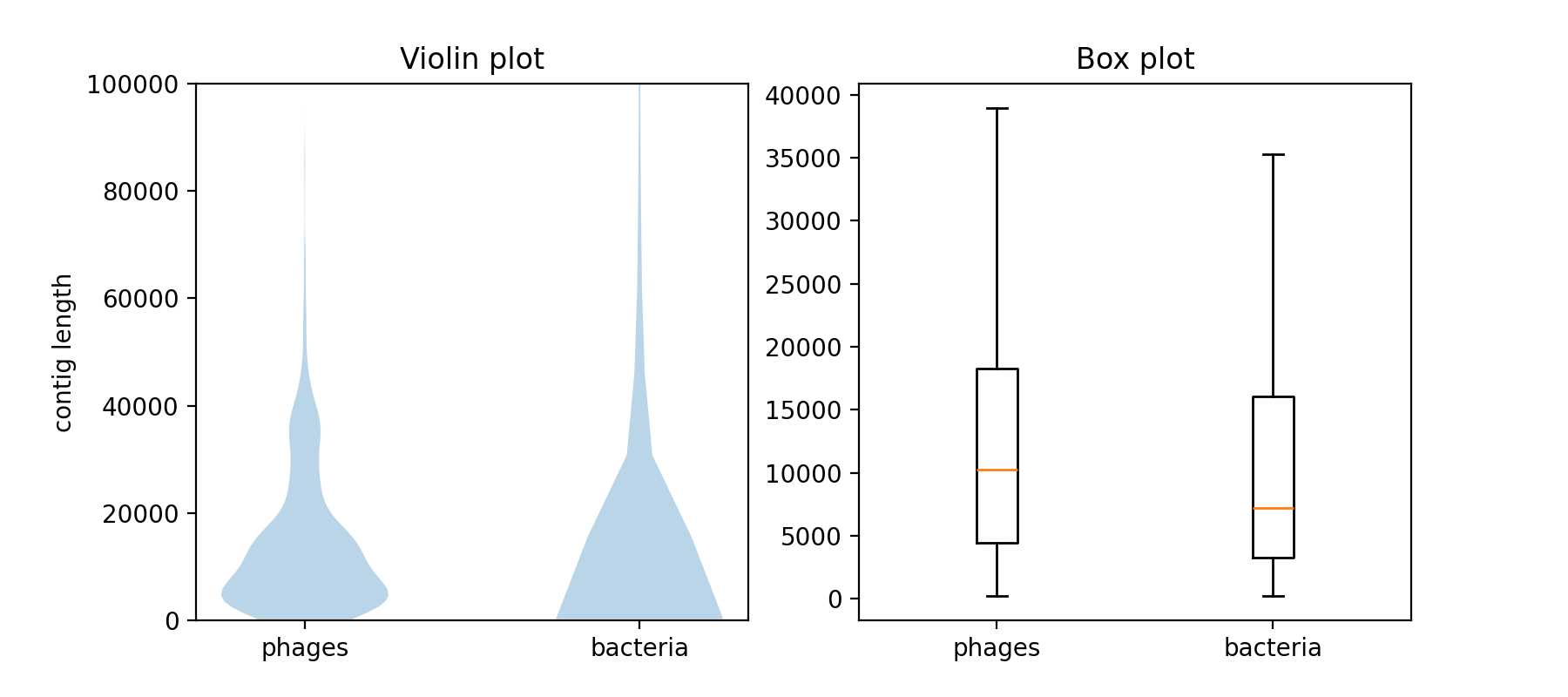
This assembly contains much longer, but also generally more contigs than the virome assembly. Use Matplotlib to visualize the distribution of the contig lengths. Use at least two plot types (e.g. histogram, violin plot, or boxplot) and adjust the plots to optimally visualize the differences in the contig length distributions. The bacterial assembly contains some very long fragments (outliers), try to find a way to deal with those.
First, you have to include Matplotlib into your virtual environment:
# activate the environment
$ source path/to/your/py3env/bin/activate

# install the packages we need
$ pip install matplotlib
Then you can write a plotting script. If you want to put multiple plots into the same figure, you can use the following lines of code:
import matplotlib as plt

# create a figure with two panels horizontally next to each other
fig, axs = plt.subplots(nrows=1, ncols=2, figsize=(9, 4))

# plot into the first (left) panel
axs[0].violinplot(list_of_datasets_to_plot)

# plot into the second (right) panel
axs[0].boxplot(list_of_datasets_to_plot)

# save the figure to a file
fig.savefig("filename.png")
python script for plotting differences in distributions
# This script takes 3 arguments. Run it:
# python your_script_file_name.py path/to/assembly1.fasta path/to/assembly2.fasta box_and_violin.png

import os, sys
from Bio import SeqIO
import matplotlib.pyplot as plt

def main():
    # take the first argument to the script as the filename to the bacterial assembly
    assembly1_filename = os.path.abspath(sys.argv[1])
    assert assembly1_filename.endswith(".fasta")

    # take the second argument to the script as the filename to the viral assembly
    assembly2_filename = os.path.abspath(sys.argv[2])
    assert assembly2_filename.endswith(".fasta")

    # set the filename of the output PNG file
    out_filename = os.path.abspath(sys.argv[3])
    assert out_filename.endswith(".png")

    # open the assembly files and get the lengths of each contig within one list
    with open(assembly1_filename) as handle:
        lengths_assembly1 = [len(record.seq) for record in SeqIO.parse(handle, "fasta")]

    with open(assembly2_filename) as handle:
        lengths_assembly2 = [len(record.seq) for record in SeqIO.parse(handle, "fasta")]

    # use pyplot to create a multi panel plot with 2 columns and 1 row. figsize is in inches...
    fig, axs = plt.subplots(nrows=1, ncols=2, figsize=(9, 4))

    # make violin plots for both lists of contig lengths
    axs[0].violinplot([lengths_assembly1, lengths_assembly2], showextrema=False)

    # add axis description and title, limit the y range for comparability
    axs[0].set_xticks([1,2], ["phages", "bacteria"])
    axs[0].set_ylim([0,100000])
    axs[0].set_title('Violin plot')

    # make box plots for both lists of contig lengths and add lables
    axs[1].boxplot([lengths_assembly1, lengths_assembly2], showfliers=False)
    axs[1].set_xticks([1,2], ["phages", "bacteria"])
    axs[1].set_title('Box plot')

    fig.savefig(out_filename, dpi=200)


if __name__ == "__main__":
    main()
Plot the difference between two assemblies
Plot the distribution of the lengths of both, the bacterial and the viral assemblies using Matplotlib. Choose at least 2 of the following:
- histogram
- boxplot
- violin plot
What are the strengths and weaknesses of your chosen visualizations? How do they compare in highlighting the differences in the length distributions of the two assemblies?
Key Points
matplotlib and pyplot provide multiple tools for the visualization of data points
Gene Calling and Functional Annotation I
Overview
Teaching: 120 min
Exercises: 60 minObjectives
Understand what is gene calling and functional annotation
Investigate the features of phages and how it impacts ORF annotation
Understand what information functional annotation can provide
![]()
Gene Finding
Once we have an assembled genome sequence (or even a contig that represents a fragment of a genome), we want to know what kind of organism the sequence belongs to (taxonomic annotation), what genes it encodes (gene annotation or gene calling), and the functions of those genes (functional annotation). Ideally, gene calling uses a good gene model that is tailored to the organism of study, but to determine the organism we need to know its genes. So it can be an iterative process. In our case, there are pretty good standard gene models available for bacteria and for phages, which we will use.
Phage genomes have specific features that are important to keep in mind. The following lecture by Dr. Robert Edwards explains these, and how they were taken into account when developing a specialized phage gene caller Phanotate.
- Click on the image to see the lecture video “Phage Genomics” by Dr. Rob Edwards (29 minutes):

The video below by Dr Evelien Adriaenssens explains more about phage genome structure and functional annotation
- Click on the image to see the lecture video “Basics of phage genome annotation & classification: getting started” by Dr Evelien Adriaenssens (68 minutes, watch from 12:02 to 30:45):

Exercise
Watch the video lectures for gene finding and functional annotation to answer the questions below:
- What is genome annotation?
- What are ORFs and why are they important in annotating genes?
- Explain the Phanotate algorithm.
- Name at least 3 features of phages should be considered when developing a phage gene annotation tool
Additional Resources
The links of Prodigal and Phanotate might also useful for answering the questions.
As additional material, the video by Dr. Katelyn McNair contains explanations of the algorithm of Phanotate. The topic is similar to the video by Dr. Robert Edwards, but more detailed about the algorithm
Functional Annotation
Once you have ORFs for your phage genomes, you might be curious to what genes they represent. Annotating genes on a genome is called functional annotation and gives insights into the phage lifestyle (lytic or lysogenic), taxonomy, hosts interactions and much more. Therefore, this is probably one of the most biologically informative and interesting steps of the viromics pipeline.
To annotate the phage genomes we will use a tool called Pharokka. Pharokka uses phannotate for the gene calling.
Exercise
The pharokka paper.
Please read the paper for pharokka - from sections 1 - 2.4 to answer the following questions:
- What genomics features are taken into account in the pharokka algorithm?
- How does pharokka assign functional annotations to ORFs using PHROGs?
- What is an HMM?
Additional Resources
The PHROG paper and the PHROGs database might also be useful for you
A caveat to pharokka
As pharokka uses PHROGs to annotate viral genomes, it is limited in the types of auxiliary metabolic genes it can assign. This limitation is set by which genes were previously classified as AMGs and therefore have a PHROG. De novo assignment of AMGs is not possible. AMGs therefore might be better assigned by using a bacterial or a combination viral+bacterial functional annotation tool like DRAM
Key Points
Genome annotation gives meaning to genomic sequences
ORFs can be predicted from start and stop codons in the genomic sequences
Phages have different genomic features than prokaryotes, which influences the design of algorithms
Tools like Phanotate are very useful to process a large amount of contigs. However, no tool is perfect, so a critical interpretation of the results is important
Functional annotation of viral genomes can give clues about viral lifestyle and host interactions
Gene Calling and Functional Annotation II
Overview
Teaching: min
Exercises: 180 minObjectives
Perform gene calling and functional annotation on the viral contigs
Running pharokka
For the functional annotation of our viral contigs, we will be using Pharokka. The “viral contigs” are the contigs we filtered yesterday (i.e. using Jaeger and CheckV)
We first have to load the appropriate conda environment
source /vast/groups/VEO/tools/anaconda3/etc/profile.d/conda.sh

conda activate pharokka_v1.7.1
The base usage for this program follows:
pharokka.py -i <fasta file> -o <output folder> -d <path/to/database_dir> -t <threads>
See the docs for the pharokka parameters
We have to add the following options:
- the pharokka database is here:
/work/groups/VEO/databases/pharokka/v1.7.1/ - To run on viral contigs from a metavirome:
-m - To also use PyHMMER
--meta_hmm - To use Phanotate for the gene prediction:
-g phanotate
Therefore your command should look like this:
pharokka.py -i filtered_assembly.fasta -o output_dir -d path/to/database -t 10 -m --meta_hmm -f -g phanotate
We recommend modifying the following SBATCH resources:
- #SBATCH –cpus-per-task=10
- #SBATCH –partition=short,standard,interactive
- #SBATCH –mem=10G
Exercise
- Run pharokka with the appropriate parameters using an sbatch script
sbatch script for pharokka
#!/bin/bash
#SBATCH --tasks=1
#SBATCH --cpus-per-task=10
#SBATCH --partition=short,standard,interactive
#SBATCH --mem=20G
#SBATCH --time=02:00:00
#SBATCH --job-name=pharokka
#SBATCH --output=./1.4_annotation/10_pharokka/pharokka.slurm.out.%j
#SBATCH --error=./1.4_annotation/10_pharokka/pharokka.slurm.err.%j

source /vast/groups/VEO/tools/anaconda3/etc/profile.d/conda.sh && conda activate pharokka_v1.7.1


database='/work/groups/VEO/databases/pharokka/v1.7.1/'
assembly='./1.3_virus_identification/40_results_filter_contigs/assembly.fasta'
outdir='./1.4_annotation/10_pharokka'

# extra options to use

# -m: run in metavirome mode (each contig is a new virus)
# --meta_hmm : also run PyHMMER on the PHROGS (richer annotations with this)
# -f: force restart the outputs
# -g: gene annotation by phanotate (default for meta mode is prodigal-gv)

pharokka.py -i $assembly -o $outdir -d $database -t 10 -m --meta_hmm -f -g phanotate
Plotting functional annotations
Choose a pet contig (or two)
Exercise - extracting contig information
- Choose a pet contig. Maybe your favourite contig number… but we recommend choosing one with high completeness and which is ‘annotation-rich’
- perhaps with many annotated genes, a crispr region, mash results (from pharokka) etc.
- Discuss with your classmates so that everybody picks a different virus one. We will continue using this “pet” contig in the future lessons also. a) Write down some information about your contig. e.g. contig length, # of genes, # of annotated genes, gc%, coding density
For the plotting we, we will still use pharokka. Pharokka’s built-in pharokka_plotter.py uses a python library called pyCirclize. You will also use this library later for the visualization homework so stay tuned!
pharokka_plotter.py requires a gff, genbank and fasta file for the viral contig. Therefore, we have to extract these from the larger pharokka.gff and pharokka.gbk outputs.
The .gff file contains information about the gene positions and strands
The .gbk file contains information about the functional annotations of each gene
The fasta file contains the nucleotide sequence
Exercise - extracting contig information
We need 3 pieces of information about your particular contig to use the pharokka plotter
- contig.gff : extracted from the pharokka.gff
- contig.gbk : extracted from the pharokka.gbk
- contig.fasta : nucl. sequence extracted from the filtered assembly
- Extract the functional annotation information for your contig from the
pharokka.gffandpharokka.gbkfiles and the contig nucleotide sequence from the fasta file
Gff and fasta files are easy to pull information from so we can just grep or sed the contig directly into an output file
Extract contig.gff
grep "contig_xxxx" pharokka.gff > contig_xxxx.gff

# for example
mkdir -p ./1.4_annotation/10_pharokka/11_selected_contig

# get the contig.gff
grep "contig_827" ./1.4_annotation/10_pharokka/pharokka.gff > ./1.4_annotation/10_pharokka/11_selected_contig/contig_827.gff
Extract contig fasta
# if your fasta file is in multi-line format
# this tells sed to print between "contig_1026" and the next ">", including both patterns
# `head` removes the last line (the second header)
sed -n '/contig_1026/,/>/p' phage_contigs.fasta | head -n -1

# for example:
sed -n '/contig_827/,/>/p' ./1.2_assembly/10_results_assembly_flye/cross_assembly/assembly.fasta | head -n -1  > ./1.4_annotation/10_pharokka/11_selected_contig/contig_827.fasta
Genbank files are a bit more difficult to extract information from but they are formatted sequentially by records. Luckily for us, there are pre-built modules in the biopython library to work with genbank files. SeqRecord and Bio.SeqIO.parse
If you head the pharokka.gbk file, you might see how the records are structured:
LOCUS       contig_1026            35733 bp    DNA     linear   PHG 06-SEP-2024
DEFINITION  contig_1026.
ACCESSION   contig_1026
VERSION     contig_1026
KEYWORDS    .
SOURCE      .
  ORGANISM  .
            .
FEATURES             Location/Qualifiers
     CDS             complement(618..749)
                     /ID="contig_1026_CDS_0001"
                     /transl_table=11
                     /phrog="No_PHROG"
                     /top_hit="No_PHROG"
                     /locus_tag="contig_1026_CDS_0001"
                     /function="unknown function"
                     /product="hypothetical protein"
                     /source="Pyrodigal-gv_0.3.1"
                     /score="3.3"
                     /phase="0"
                     /translation="MTRWNTTLAVYEIWTGTQWQAVASSTYSINYLIVAGGASGAHY*"

See if you can write a script to extract the genbank record for your contig using this module - for clues - see solution below!
The whole contig is called a “record” - see the biopython SeqRecord class page for what each element in the record is called, use Bio.SeqIO.parse to iterate through these records and Bio.SeqIO.write to write out the record you want.
biopython script to extract contig.gbk (genbank)
#!/usr/bin/python3

from Bio import SeqIO
import sys

# read files in as variables
input_gbk = sys.argv[1]
output_gbk = sys.argv[2]
contig = sys.argv[3]

# parse the genbank and write output
for record in SeqIO.parse(input_gbk, "genbank"):
   # print(record.id)
   if record.id == contig:
       SeqIO.write(record, output_gbk, "genbank")
sbatch script to run your python script
#!/bin/bash
#SBATCH --tasks=1
#SBATCH --cpus-per-task=1
#SBATCH --partition=short,standard,interactive
#SBATCH --mem=2G
#SBATCH --time=00:01:00
#SBATCH --job-name=py_script
#SBATCH --output=./1.4_annotation/10_pharokka/extract_contigs.slurm.out.%j
#SBATCH --error=./1.4_annotation/10_pharokka/extract_contigs.slurm.err.%j

# activate the python virtual environment with the packages we need
source ./py3env/bin/activate

# change the output and contig names accordingly
python3 python_scripts/annotation/extract_contig_gbk.py pharokka.gbk output_contig.gbk contig_xxxx
Plot your contigs!
Once we have our fasta, gff and genbank files, we can use pharokka_plotter.py to plot our pet contig. pharokka_plotter.py requires the same conda environment as pharokka. So, to to activate the environment use the same commands you used for pharokka. Feel free to experiment with the different options given in the manual. The base usage is:
pharokka_plotter.py -i input.fasta -n pharokka_plot --gff pharokka.gff --genbank pharokka.gbk
You no longer need the pharokka database and we recommend modifying the following SBATCH parameters #SBATCH --mem=10G
Exercise - plotting
- Plot the genome annotations for your pet contig
Make sure to add your plot into your lab book!
sbatch script for all the extraction steps + pharokka_plotter
#!/bin/bash
#SBATCH --tasks=1
#SBATCH --cpus-per-task=10
#SBATCH --partition=short,standard,interactive
#SBATCH --mem=10G
#SBATCH --time=2:00:00
#SBATCH --job-name=pharokka_1
#SBATCH --output=./1.4_annotation/10_pharokka/pharokka_plotter.slurm.out.%j
#SBATCH --error=./1.4_annotation/10_pharokka/pharokka_plotter.slurm.err.%j

assembly='./1.2_assembly/10_results_assembly_flye/cross_assembly/assembly.fasta'
outdir='./1.4_annotation/10_pharokka/11_selected_contig'

mkdir -p $outdir

# get the contig.gff and contig.fasta
grep "contig_827" ./1.4_annotation/10_pharokka/pharokka.gff > $outdir/contig_827.gff

sed -n '/contig_827/,/>/p' $assembly | head -n -1  > $outdir/contig_827.fasta

# next, we get the contig.gbk using a python script
# change the names accordingly

# activate the python virtual environment with the packages we need
source ./py3env/bin/activate

# the inputs for the following python script should be
# python3 script.py input.gbk output.gbk contig_name
input_gbk='./1.4_annotation/10_pharokka/pharokka.gbk'
output_gbk='./1.4_annotation/10_pharokka/11_selected_contig/contig_827.gbk'
name='contig_827'

python3 python_scripts/annotation/extract_contig_gbk.py $input_gbk $output_gbk $name

# Then we run pharokka plotter on our selected contig

source /vast/groups/VEO/tools/anaconda3/etc/profile.d/conda.sh && conda activate pharokka_v1.7.1

# define all your file paths for readability
outdir='./1.4_annotation/10_pharokka/11_selected_contig/'

fasta='./1.4_annotation/10_pharokka/11_selected_contig/contig_827.fasta'
gff='./1.4_annotation/10_pharokka/11_selected_contig/contig_827.gff'
gbk='./1.4_annotation/10_pharokka/11_selected_contig/contig_827.gbk'

pharokka_plotter.py -i $fasta -n $outdir/pharokka_plot --gff $gff --genbank $gbk
The final plot might look something like this:
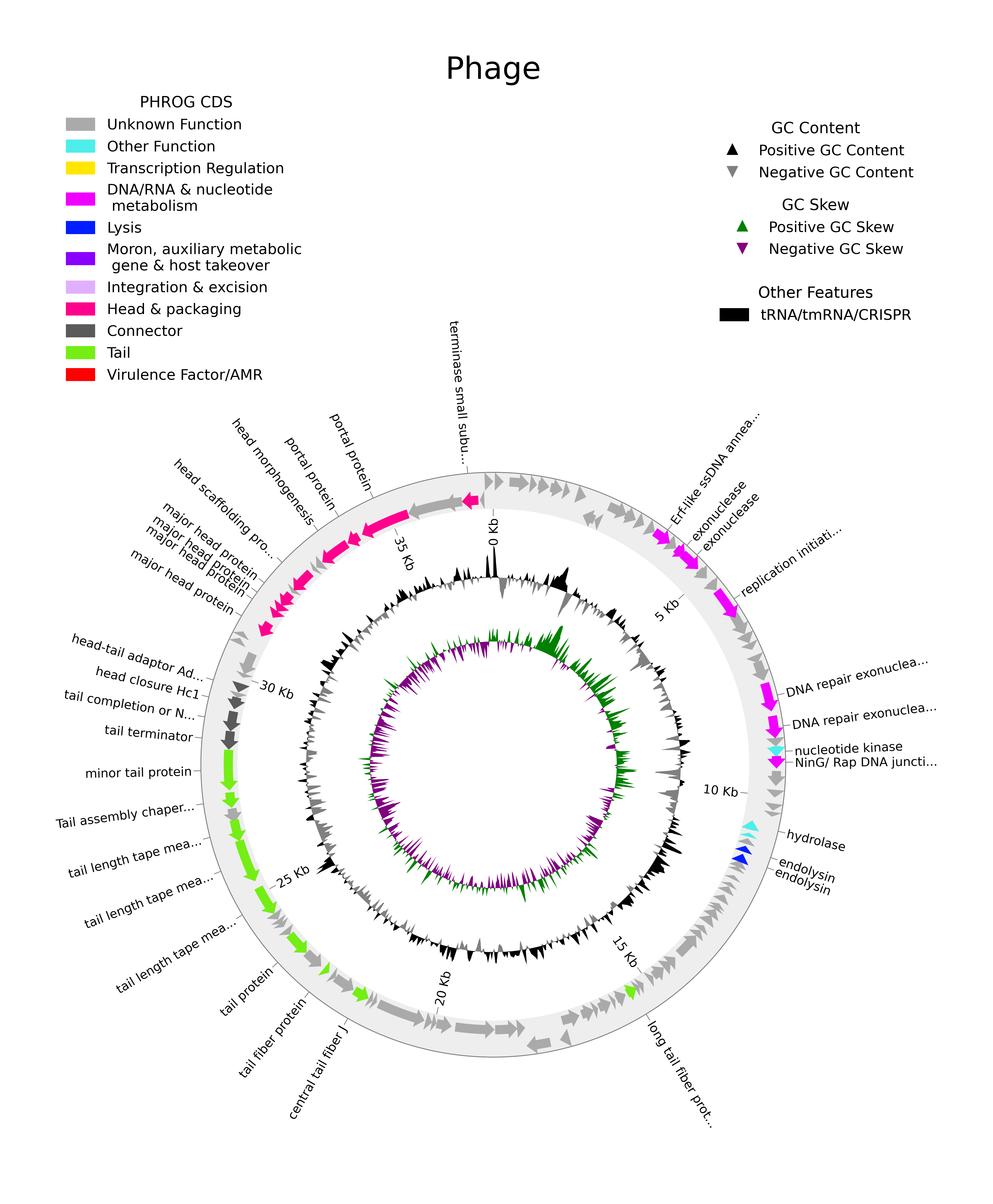
Interpreting your contig
With functional annotation we can begin to get an insight into our viruses to piece together information about their lifestyles, hosts interactions etc, what type of genes they have. You’ll find that most genes on viral contigs are not actually annotated - this is because 1) viruses evolve very quickly and assigning gene annotations by homology is difficult, and 2) viruses are highly mosaic - they pick up and lose genes from their hosts and other viruses, meaning not all viruses have all the same genes and viral gene databases do not always account for their variability. The creation of newer tools like phold aid in this by using structural homologs to assign gene annotation.
Note : We have phold installed on Draco, if you would like to experiment with it for your project! For example, you might pick a contig that is NOT well annotated and see how many extra genes you can annotate using structural homology
Exercise - Interpret your contigs
- How many structural genes are annotated?
- Describe at least 2 different types of structural genes a) Where are they placed in your genome? b) To which part of phage structure do they belong? (capsid, tail etc) c) What other viruses have these structural features?
- How many replication genes are annotated?
- These could be genes related to transcriptional regulation, DNA/RNA metabolism lysis etc
- Describe the role of 1 replication gene a) What is the function of the gene? b) What part of the replication cycle is it used? c) How does it interact with the host genes (if they do)
- Describe 1 or more interesting genomic features
- CRISPR arrays, tRNA, virulence factors etc
- To the best of your ability, infer how this virus might be interacting with its host.
- You might investigate clues temperate/lytic lifestyles, auxiliary metabolic genes, anti-crisprs etc
Key Points
Functional annotation of viral genomes can give clues about viral lifestyle and host interactions
Visualizing an annotated viral genome
Overview
Teaching: min
Exercises: 90 minObjectives
Use Python to draw a map of a viral genome
Visualize gene overlap and direction
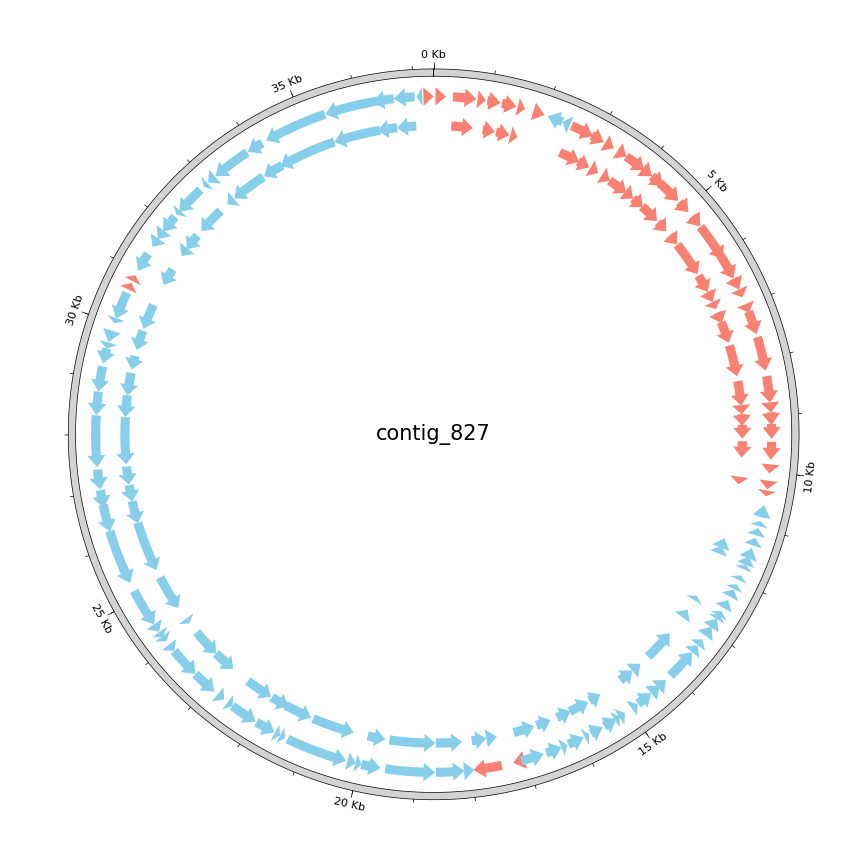
Next, we will visualize the differences in ORFs called by the two tools phannotate and prodigal-gv. Phannotate is used by Pharokka, which we ran to find genes and annotate them with funktions today. Yesterday we used CheckV to estimate the completeness of viral contigs. This tool is based on gene annotations found by prodigal-gv. To illustrate the difference between the two methods, we will plot the sets of genes used by both tools similar to the plots you generated today using Pharokka, which are based on the python package pyCirclize. The pyCirclize package provides tools to generate high-quality plots of annotated genomes in a circular layout, and allows for adding various data elements. Check the GitHub page to get an idea of its possibilities. To use the package, you have to install it into your virtual environment:
# activate the environment
$ source path/to/your/py3env/bin/activate

# install the packages we need
$ pip install pyCirclize
You can get some examples of how to use the package here.
Starting from the first example, the Circos plot of the Enterobacter phage, adjust it to show both Phanotate
and CheckV ORFs on your pet phage genome. We want to compare the differences in ORF calling.
The information about the ORFs used by CheckV can be found in the tmp folder in your CheckV results (gene_features.tsv).
Exercise - plot two sets of gene predictions
Optional: Think about a way to convert the information in the TSV file into something parsable by pyCirclize and write a script for plotting the two sets of ORFs.
You can use the solution for the optional task above to create a .gff file from the gene predictions contained in the
gene_features.tsvfile of CheckV. If you run the script(s) on Draco, please remember to use slurm. The plotting script should not need much memory and can run on a single core.
Python script for converting tabular annotations into the GFF format
# This script expects three parameters to be passed to it. The path to CheckV's gene_features.tsv,
# the filename of the output .gff file and the name of the contig to be exported to gff.

import pandas as pd
import gffutils.gffwriter as gw
import gffutils.feature as gf
import os, sys

def main():

  # read parameters passed to the script. It ex
  in_file = os.path.abspath(sys.argv[1])
  assert in_file.endswith(".tsv")

  out_file = os.path.abspath(sys.argv[2])
  writer = gw.GFFWriter(out_file)

  contig_id = sys.argv[3]

  # read the .tsv file into a pandas dataframe (sep="\t" reads tab-separated files)
  df = pd.read_csv(in_file, sep="\t")
  # select the ORFs with the specified contig name
  df = df.loc[df["contig_id"] == contig_id]

  # iterate through the ORFs of the selcted contig
  for index, row in df.iterrows():
    # convert the strand integer into GFF-compatible "+" and "-"
    if row["strand"] == 1: strand = "+"
    else: strand = "-"
    # use gfutils to create a GFF feature from the information in the dataframe and append it to the output file
    f = gf.Feature(seqid=row["contig_id"], featuretype="CDS", start=row["start"], end=row["end"], strand=strand)
    writer.write_rec(f)

  # close the writer to flush the writing buffer and properly finish the file
  writer.close()

if __name__ == "__main__":
    main()
python script for plotting ORFs with pyCirclize
# This script expects four paramerters passed to it. 1. The filename of the .gff file you generated with the above script,
# 2. the gff created by phannotate during todays practical session, 3. the filename of the output .png file and 4. the name
# of the contig you want to plot

from pycirclize import Circos
from pycirclize.parser import Gff
import os, sys

def main():
  # read the parameters passed to the script (see first comment for details)
  prodigal_filename = os.path.abspath(sys.argv[1])
  assert prodigal_filename.endswith(".gff")

  phanotate_filename = os.path.abspath(sys.argv[2])
  assert phanotate_filename.endswith(".gff")

  out_filename = os.path.abspath(sys.argv[3])
  assert out_filename.endswith(".png")

  contig_id = sys.argv[4]

  # use pycirclize's GFF parser to read the two input GFF files
  prodigal_gff = Gff(prodigal_filename)
  phanotate_gff = Gff(phanotate_filename)

  # Initialize circos sector by genome size
  circos = Circos(sectors={phanotate_gff.name: phanotate_gff.range_size})
  circos.text(contig_id, size=15)
  sector = circos.sectors[0]

  # Outer track: add size marks for the genome's length
  outer_track = sector.add_track((98, 100))
  outer_track.axis(fc="lightgrey")
  outer_track.xticks_by_interval(5000, label_formatter=lambda v: f"{v / 1000:.0f} Kb")
	outer_track.xticks_by_interval(1000, tick_length=1, show_label=False)

  # Plot forward & reverse CDS genomic features and color them differently for phannotate's ORF predictions
  cds_track = sector.add_track((90, 95))
  cds_track.genomic_features(phanotate_gff.extract_features("CDS", target_strand=1), plotstyle="arrow", fc="salmon")
  cds_track.genomic_features(phanotate_gff.extract_features("CDS", target_strand=-1), plotstyle="arrow", fc="skyblue")

  # Plot forward & reverse CDS genomic features and color them differently for prodigal's ORF predictions
  cds_track = sector.add_track((82, 87))
  cds_track.genomic_features(prodigal_gff.extract_features("CDS", target_strand=1), plotstyle="arrow", fc="salmon")
  cds_track.genomic_features(prodigal_gff.extract_features("CDS", target_strand=-1), plotstyle="arrow", fc="skyblue")

  # save plot to file
  circos.savefig(out_filename)

if __name__ == "__main__":
  main()
sbatch script for submitting the plotting script
#!/bin/bash
#SBATCH --tasks=1
#SBATCH --cpus-per-task=1
#SBATCH --partition=short
#SBATCH --mem=2G
#SBATCH --time=00:01:00
#SBATCH --job-name=plot
#SBATCH --output=./1.4_annotation/20_plot_viral_genome/viral_genome.slurm.%j.out
#SBATCH --error=./1.4_annotation/20_plot_viral_genome/viral_genome.slurm.%j.err

# activate the python virtual environment with the packages we need for plotting
source ./py3env/bin/activate

mkdir -p ./1.4_annotation/20_plot_viral_genome/

# define an array with contig ids to plot
declare -a arr=("contig_827" "contig_827")

features='./1.3_virus_identification/20_results_assessment_checkv/cross_assembly/tmp/gene_features.tsv'
outdir='./1.4_annotation/20_plot_viral_genome'
pharokka_dir='./1.4_annotation/10_pharokka/11_selected_contig'

# loop through the array
for contig in "${arr[@]}"
do
      echo $contig
      echo "$contig"
      # run the python script wich extracts the prodigal-gv-based annotations from the CheckV output
      # in this solution, the script expects three parameters:
      # first: the filname of the table generated by CheckV
      # second: the output filename for the filtered gff file
      # third: the contig id to filter for
      python python_scripts/annotation/10_table_to_gff.py $features $outdir/$contig.gff $contig

      # run the python script wich plots the two annotations in a circle
      # in this solution, the script expects four parameters:
      # first: the gff file of the prodigal-gv-based annotation created from CheckV's gene_features.gff
      # second: the gff file created by phanotate
      # third: the output file name
      # fourth: the contig id to write into the plot

      python python_scripts/annotation/10_viral_genome.py $outdir/$contig.gff $pharokka_dir/$contig.gff $outdir/"$contig"_circos.png $contig
done

deactivate
Compare the annotations
Describe the differences between the two gene annotations based on the plots you created. Does the visualization confer these differences well?
Key Points
The pyCirclize package provides tools for plotting genomic data, e.g., the set of genes, in a circular layout.
Host Prediction I
Overview
Teaching: 60 min
Exercises: 120 minObjectives
Understand how biological information is used to predict hosts
Understand the difficulties with host prediction
Learn about the new techniques that are being used for host prediction
![]()
Host prediction lecture
Listen to lecture by Varada and Malte (pay attention!!!) slides for host prediction
Questions
- What are some biological interactions viruses have with their hosts? (hint: start with the infection cycle)
Pick one classical host prediction method:
- In brief, explain how this works
- What is the major challenge with this method?
- How can you be confident in your host prediction?
- Evaluate the following scenarios: a) Two viral contigs match to the same host during the host prediction b) One viral contig matches 2 hosts: s__Salinibacter ruber and s__Longimonas halophila
For the hands-on part - we will be using a tool called RaFAH. This tool uses random forest model machine learning models to predict hosts for phages. They train the ML model using the protein content of viral sequences and compare it with manually curated classical host predictions (CRISPR sequences, tRNA and homology based matches) and related other tools. Have a look into the RaFAH paper and focus on the introduction and Figures 1 and 2.
Questions
- Briefly discribe how RaFAH derives its predictions from a genome sequence.
RaFAH produces a probability score for each host genus in its training set and reports the genus with the maximum probability. In Figure 2, you can find how this score relates to precision and recall for the test dataset the authors used.
- Decide, which probability score you would use as a cutoff for predictions you would trust. Explain your decision.
Additional resources
- IBM link on Random Forest (RF): introduces RF and decision trees in a short and simple way
- Chapter on RF for Bioinformatics: explains how RF measures feature importance and describes Bioinformatic applications
- Chapter on Decision Trees and RF: describes decision trees and RF by direct application in python. Also, if you want a great introduction to machine learning in general and python programming, take a look at the whole book by Jake VanderPlas, which is freely available online
Key Points
Host Prediction II
Overview
Teaching: 0 min
Exercises: 240 minObjectives
Run RaFAH to predict a host genus for each contig.
Run BLASTn to find homologies between metagenome and metavirome.
Host prediction
Today, we will use the tool RaFAH to predict a genus of a putative host for our contigs. The tool predicts proteins in each viral sequence and then assigns them to a set of orthologous groups. The annotated proteins are then used to predict a host genus with a pretrained random forest model. This model matches the set of proteins with host proteins it was trained on.
After running RaFAH, we will compare the resulting prediction with the bacterial metagenome you briefly analyzed in one of last weeks homeworks. The bacterial metagenome was taxonomically annotated using GTDB. We will get into taxonomic classification of viruses tomorrow, for today it is important to know that there are different methods of taxonomic classification. RaFAH uses the NCBI taxonomy, so we will have to translate the output of RaFAH into the GTDB taxonomy to be able to compare the predictions with our bacterial metagenome.
Next, we will use BLAST as an alternative way of linking viruses to their hosts. With BLAST, we will align our viral contigs to putative bacterial and archael genomes (Metagenome-Assembled-Genomes, MAGS) to find sequence matches between the viruses and potential hosts.
Finally, we will combine the results from RaFAH and BLAST to compare the two methods and see how well they agree.
RaFAH
Exercise - Use RaFAH to predict hosts for our contigs
RaFAH requires a single file for each contig to run. You first have to write a python script which separates the combined assembly into single files. You can use the package biopython installed in your virtual environment for this:
import os, sys
from Bio import SeqIO

# define file paths from the arguments
...

# loop through the records in the combined assembly
with open(assembly_path) as handle:
    for record in SeqIO.parse(handle, "fasta"):
        # set a filename per record
        out_fasta = os.path.join(out_dir, f"{record.id}.fasta")
        # write the record to the file
        with open(out_fasta, "w") as fout:
            SeqIO.write([record], fout, "fasta")
Next, you will write a python script, which translates the host genus predictions from the NCBI taxonomy into the GTDB taxonomy. You can copy the translation table from this location on draco:
$ cp /work/groups/VEO/shared_data/Viromics2024Workspace/2.1_host_prediction/ncbi_to_gtdb.csv ./2.1_host_prediction/10_rafah/ncbi_to_gtdb.csvThere are hundreds of thousands of taxa in both taxonomy schemes, so we need to efficiently map one onto the other. Here are some hints:
import os, sys
import pandas as pd

# Extract the genus part of the NCBI taxonomy.
# This should correspond to RaFAH's output
def get_ncbi_genus(s):
    for ss in s.split(";"):
        if ss.startswith("g__"): return ss[3:]
    return "none"

# Extract the complete taxonomic classification up to genus from GTDB
def get_gtdb_upto_genus(s):
    return s.split(";s__")[0]

# set or get filenames from sys.argv and read tables with pandas
...

# create a dictionary for efficient mapping between the two taxonomies
translation_dict = {get_ncbi_genus(r["ncbi_taxonomy"]):get_gtdb_upto_genus(r["gtdb_taxonomy"]) for i, r in translate_df.iterrows()}

# use the dictionary to translate the predictions in the RaFAH output table
...
You can run the scripts in the same sbatch script as RaFAH. Remember to source and deactivate our python virtual environment accordingly. Here you can find a description of the parameters you can pass to RaFAH (the page is a bit hard to read). The tool is programmed in perl and you can find it here on draco:
# activate the conda environment with the dependencies RaFAH requires
source /vast/groups/VEO/tools/miniconda3_2024/etc/profile.d/conda.sh && conda activate perl_v5.32.1

# set a variable to call the RaFAH script
rafah='/home/groups/VEO/tools/rafah/RaFAH.pl'

# create an output folder or use the one you set for the slurm logs:
mkdir 10_results_hostprediction_rafah

# run RaFAH with the appropriate file paths and arguments
perl "$rafah" --predict --genomes_dir 10_results_hostprediction_rafah/split_contigs --extension .fasta
RaFAH is computationally expensive and can use multiple threads. We recommend you set the following sbatch parameters:
- #SBATCH –cpus-per-task=32
- #SBATCH –partition=standard,short
- #SBATCH –mem=50G
RaFAH uses the random forest model to compute a probability for all host genuses included in its training. You can find these probabilities in the output file
*Host_Predictions.tsv. The file*Seq_Info_Prediction.tsvcontains per contig the genus with the highest probability.
- How many contigs have a probability score larger than your chosen cutoff?
- Does the probability score relate to the completeness of the contigs? (qualitative answer)
python script for splitting the assembly into separate files
import os, sys
from Bio import SeqIO

def main():

    # define file paths from the arguments
    assembly_path = os.path.abspath(sys.argv[1])
    assert assembly_path.endswith(".fasta")

    # set an output directory and create it if it does not exist
    out_dir = os.path.abspath(sys.argv[2])
    if not os.path.exists(out_dir): os.makedirs(out_dir)

    # loop through the records in the combined assembly
    with open(assembly_path) as handle:
        for record in SeqIO.parse(handle, "fasta"):
            # set a filename per record
            out_fasta = os.path.join(out_dir, f"{record.id}.fasta")
            # write the record to the file
            with open(out_fasta, "w") as fout:
                SeqIO.write([record], fout, "fasta")

if __name__ == "__main__":
    main()
python script for translating NCBI genus IDs to GTDB
import os, sys
import pandas as pd

# Extract the genus part of the NCBI taxonomy.
# This should correspond to RaFAH's output
def get_ncbi_genus(s):
    for ss in s.split(";"):
        if ss.startswith("g__"): return ss[3:]
    return "none"

# Extract the complete taxonomic classification up to genus from GTDB
def get_gtdb_upto_genus(s):
    return s.split(";s__")[0]

def main():

    # set the filename of the rafah output file containing the best prediction per contig
    rafah_filename = os.path.abspath(sys.argv[1])
    assert rafah_filename.endswith(".tsv")

    # set the filename of the translation table with NCBI and GTDB taxonomic IDs
    translation_filename = os.path.abspath(sys.argv[2])
    assert translation_filename.endswith(".csv")

    # set the output filename
    out_filename = os.path.abspath(sys.argv[3])
    assert out_filename.endswith(".csv")

    # read the input tables using pandas
    translate_df = pd.read_csv(translation_filename)
    rafah_df = pd.read_csv(rafah_filename, sep='\t')

    # we are only interested in the first 3 columns
    rafah_df = rafah_df.iloc[:, :3]

    # create a dictionary for efficient matching of NCBI to GTDB
    translation_dict = {get_ncbi_genus(r["ncbi_taxonomy"]):get_gtdb_upto_genus(r["gtdb_taxonomy"]) for i, r in translate_df.iterrows()}

    # translate all NCBI genus predictions to GTDB.
    # We don't manipulate the table while iterating over it because this could lead to problems.
    translated_hosts = []
    for i, row in rafah_df.iterrows():
        translated_hosts.append(translation_dict[row["Predicted_Host"]] if row["Predicted_Host"] in translation_dict else "no_translation")

    # add the translated predictions to the dataframe and save the table.
    rafah_df["Predicted_Host"] = translated_hosts
    rafah_df.to_csv(out_filename,index=False)

if __name__ == "__main__":
    main()
sbatch script for host prediction with RaFAH
#!/bin/bash
#SBATCH --tasks=1
#SBATCH --cpus-per-task=32
#SBATCH --partition=short,standard
#SBATCH --mem=50G
#SBATCH --time=02:00:00
#SBATCH --job-name=rafah
#SBATCH --output=./2.1_host_prediction/10_rafah/rafah.slurm.%j.out
#SBATCH --error=./2.1_host_prediction/10_rafah/rafah.slurm.%j.err

assembly='./1.3_virus_identification/40_results_filter_contigs/assembly.fasta'
contigs='./2.1_host_prediction/10_rafah/split_contigs'

# RaFAH expects each genome in a separate file. Activate our virtual environment
# and run a python script to split our filtered assembly into single files
source ./py3env/bin/activate

# The script requires the assmbly path and a directory for outputting the contigs
python ./python_scripts/host_prediction/10_split_assembly_file.py $assembly $contigs

# deactivate the python environment, just to be sure not to cause problems with the conda environment RaFAH needs
deactivate

# activate the conda environment with the dependencies RaFAH requires
source /vast/groups/VEO/tools/miniconda3_2024/etc/profile.d/conda.sh && conda activate perl_v5.32.1

# set a variable to call the RaFAH script
rafah='/home/groups/VEO/tools/rafah/RaFAH.pl'

# rafah parameters (https://gensoft.pasteur.fr/docs/RaFAH/0.3/)
# --predict: run the pipeline for predicting hosts
# --genomes_dir: the directory with the separate files for each contig
# --extension: the extension of the contig files
# --file_prefix: can specify an output dir here and "run name" (rafah_1) here

perl "$rafah" --predict --genomes_dir $contigs --extension .fasta --file_prefix ./2.1_host_prediction/10_rafah/rafah_1

# deactivate RaFAH's conda environment
conda deactivate

# Our python script for translating the Taxonomy needs our python environment again
source ./py3env/bin/activate

# set the path to the table with the translation between NCBI and GTDB and to RaFAH output
translation='./2.1_host_prediction/10_rafah/ncbi_to_gtdb.csv'
rafahtable='./2.1_host_prediction/10_rafah/rafah_1_Host_Predictions.tsv'

# run our script with the appropriate file names as parameters
python3 ./python_scripts/host_prediction/20_translate_taxonomy.py $rafahtable $translation ./2.1_host_prediction/10_rafah/rafah_1_Host_Predictions_gtdb.csv

deactivate
Host Prediction using Blastn
While RaFAH uses a database of reference bacterial/archaeal genomes to find hosts, these bacteria/archaea may or may not be in your samples. One of the simplest ways to look for potential hosts is to do a quick blastn. Viral genomes often contain fragments of host DNA, for example an auxiliary metabolic gene. Conversely, viral DNA can also be found in host genomes; e.g. prophages, CRISPR spacers, fragments of viral genes, tRNAs etc.
For this task, we assembled metagnome-assembled-genomes (MAGs or bins) of the prokaryotic community from the same three samples given to you. This resulted in 110 MAGs. However, not all of these are complete and many are contaminated. After filtering for a completeness >= 50% and a contamination <= 6%, 19 “good MAGs” remained.
These “good MAGs” were concatenated and are located /work/groups/VEO/shared_data/Viromics2024Workspace/test_run/2.1_host_prediction/20_blastn/good_bins_all.fa. These MAGs will be the “database” against which we align our viral contigs (query sequences)
You also require the GTDB taxonomic classifications for the bins. These are located /work/groups/VEO/shared_data/Viromics2024Workspace/2.3_bacterial_binning/40_gtdbtk/results/gtdbtk.bac120.summary.tsv
Exercise - copy the MAGs and the gtdb bin classification over
Please copy this fasta file into your own directory
# make a new directory for this analysis
mkdir ./2.1_host_prediction/20_blastn/

# copy over the good MAGs
cp /work/groups/VEO/shared_data/Viromics2024Workspace/test_run/2.1_host_prediction/20_blastn/good_bins_all.fa ./2.1_host_prediction/20_blastn/

# copy over the taxonomic classification for the MAGs
cp /work/groups/VEO/shared_data/Viromics2024Workspace/2.3_bacterial_binning/40_gtdbtk/results/gtdbtk.bac120.summary.tsv ./2.1_host_prediction/20_blastn/gtdbtk.bac120.summary.tsv
Next, we will create a custom blast database using our MAGs fasta file and use blastn (nucleotide-nucleotide) to do the alignment
Exercise - makeblastdb and blastn
Create an sbatch script for the makeblastdb and blastn
- makeblastdb is located at
/home/groups/VEO/tools/blast/v2.14.0/bin/makeblastdb- blastn is located at
/home/groups/VEO/tools/blast/v2.14.0/bin/blastn- A conda environment is NOT required for this tool!
The basic usage for the makeblastdb and blastn are the following
NOTE: the database you create in makeblastdb has to be fed into blastn
# make a custom database
makeblastdb -in mags_file.fasta -out  mags_file.fasta -dbtype nucl

# run blastn with the file.fasta database
blastn -db mags_file.fasta -query filtered_cross_assembly.fasta -out viral_contigs_vs_bins_blastn.out -num_threads 32 -outfmt 6
Resources for blastn can vary! Large databases require a lot of computational power and will take a long time but luckily our task is very small. We recommend the following resources
#SBATCH –cpus-per-task=32
#SBATCH –partition=short,standard
#SBATCH –mem=5G
#SBATCH –time=01:00:00
-outfmt 6 : is an output format that is tabular. Your output contains the following 12 columns in THIS order
query, subject, pid, aln_length, mismatch, gapopen, qstart, qend, sstart, send, evalue, bitscore
query : query id - this is your viral contig
subject : subject id - this is the bin and contig it matches
pid : percent id of the match
aln_length : alignment length
mismatch : number of mismatches
gapopen : number of gaps
qstart, qend : start and end positions of query sequence
sstart, send : start and end positions of subject sequence
evalue : expect value (the lower, the better)
bitscore : a score based on gaps, mismatches, % id and alignment length
More resources for blast output formats here and blast manual
sbatch script for blast tasks
#!/bin/bash
#SBATCH --tasks=1
#SBATCH --cpus-per-task=32
#SBATCH --partition=short,standard
#SBATCH --mem=5G
#SBATCH --time=01:00:00
#SBATCH --job-name=blastn
#SBATCH --output=./2.1_host_prediction/20_blastn/blastn.slurm.%j.out
#SBATCH --error=./2.1_host_prediction/20_blastn/blastn.slurm.%j.err

# the blast tools
makeblastdb='/home/groups/VEO/tools/blast/v2.14.0/bin/makeblastdb'
blastn='/home/groups/VEO/tools/blast/v2.14.0/bin/blastn'

# the query (filtered cross assembly) and subject (MAGs fasta)
assembly='./1.3_virus_identification/40_results_filter_contigs/assembly.fasta'
bins_fasta='./2.1_host_prediction/20_blastn/good_bins_all.fa'

$makeblastdb -in $bins_fasta -out $bins_fasta -dbtype nucl

$blastn -db $bins_fasta -query $assembly -out ./2.1_host_prediction/20_blastn/viral_contigs_vs_bins_blastn.out -num_threads 32 -outfmt 6
Exercise - analyzing blast results
- How many total hits did you get from blastn?
- How many of these hits would you trust?
- How many unique viral contigs were you able to get host predictions for from blastn?
- Was there cases where 1 viral contig hit multiple MAGs?
a) which interaction would you then trust?
Combining results for blast and RaFAH
Now we can write a python script to combine the results from RaFAH and blastn to compare the host predictions from different method. You might use pandas dataframes and pd.join or pd.merge to write this.
You will need the following 3 files:
- the blast output:
./2.1_host_prediction/20_blastn/viral_contigs_vs_bins_blastn.outfile - the taxonomic classifications for the MAGs:
./2.1_host_prediction/20_blastn/gtdbtk.bac120.summary.tsv - the rafah results with the converted taxonomy:
./2.1_host_prediction/10_rafah/rafah_1_Host_Predictions_gtdb.csv
py script for merging the blastn and rafah results
import pandas as pd
import sys

# read in the files
blast = sys.argv[1]
taxa = sys.argv[2]
rafah = sys.argv[3]
out = sys.argv[4]

df_rafah = pd.read_csv(rafah, header=0)
print(df_rafah)

df_bins_gtdb = pd.read_csv(taxa, sep='\t' ,header=0)
print(df_bins_gtdb)

df_blast = pd.read_csv(blast, sep='\t', header=None,
                      names=['query', 'subject', 'pid', 'aln_length', 'mismatch', 'gapopen', 'qstart', 'qend', 'sstart', 'send', 'evalue', 'bitscore'])
print(df_blast.head(n=10))


# add MAG taxonomy to the blast results
df_blast['bin'] = df_blast['subject'].str.split('.fa').str[0]
print(df_blast.head(n=10))

df_blast_gtdb_merged = df_blast.merge(df_bins_gtdb[['user_genome','classification']], how='left', left_on='bin', right_on='user_genome')
print(df_blast_gtdb_merged.head(n=10))

# merge blast results with rafah
df_blast_gtdb_rafah_merged = df_blast_gtdb_merged.merge(df_rafah,how='left',left_on='query',right_on='Sequence',suffixes=(None,'_rafah'))
df_blast_gtdb_rafah_merged

# select relevant columns
df_blast_gtdb_rafah_merged=df_blast_gtdb_rafah_merged[['query', 'subject', 'pid', 'aln_length', 'mismatch', 'gapopen', 'qstart', 'qend', 'sstart', 'send', 'evalue', 'bitscore', 'bin',	'classification','Predicted_Host', 'Winner_Score']]

# rename the columns to meaningful headers
df_blast_gtdb_rafah_merged = df_blast_gtdb_rafah_merged.rename(columns = {'query':'viral_contig', 'subject':'host_bin_contig','bin':'host_bin','classification':'blast_predicted_host','Predicted_Host':'rafah_predicted_host', 'Winner_Score':'rafah_score'})

print(df_blast_gtdb_rafah_merged)

# write out to a csv
df_blast_gtdb_rafah_merged.to_csv(out,index=False)
sbatch script for blast tasks
#!/bin/bash
#SBATCH --tasks=1
#SBATCH --cpus-per-task=10
#SBATCH --partition=short
#SBATCH --mem=5G
#SBATCH --time=01:00:00
#SBATCH --job-name=combine
#SBATCH --output=./2.1_host_prediction/30_combined_results/combine.slurm.%j.out
#SBATCH --error=./2.1_host_prediction/30_combined_results/combine.slurm.%j.err

# Our python script for combining blastn and rafah needs our python environment again
source ./py3env/bin/activate

# file paths
blast='./2.1_host_prediction/20_blastn/viral_contigs_vs_bins_blastn.out'
gtdb='./2.1_host_prediction/20_blastn/gtdbtk.bac120.summary.tsv'
rafah='./2.1_host_prediction/10_rafah/rafah_1_Host_Predictions_gtdb.csv'
output='./2.1_host_prediction/30_combined_results/combined_blast_rafah_host_predictions.csv'

python3 ./python_scripts/host_prediction/30_combine_host_prediction.py $blast $gtdb $rafah $output
Exercise - comparing RaFAH and blast results
- For how many host predictions, do RaFAH and blastn agree and upto which taxonomic level?
- Are you able identify CRISPRs or integrated phage genomes?
a) Explain your decision
b) How might you confirm your CRISPR/prophage identification?- Pick one example where you would trust RaFAH predictions more and another where you would trust blast predictions more and explain why.
Key Points
RaFAH uses a random forest model to predict hosts to the genus level for phages
RaFAH returns a probability for each host genus it can predict.
Blastn between the viral and prokaryotic fractions can be used as a quick method for host prediction
Machine learning and classical host prediction methods have a trade-off between recall and sensitivity
Viral taxonomy and phylogeny I
Overview
Teaching: 60 min
Exercises: 120 minObjectives
Understand the differences between taxonomic approaches for viral and cellular organisms
Explain the challenges with viral taxonomy, and how they may be overcome
![]()
How are viruses taxonomically classified?
A widely accepted approach for taxonomic classification is by selecting a marker gene that is shared by all organisms, creating a multiple sequence alignment and phylogenetic tree, and identifying taxa as characteristic branches or lineages in the tree. This approach can be applied to all cellular organisms including bacteria, archaea, and eukaryotes, particularly with marker genes functioning in the ribosome. But only to subgroups of viruses, as no marker gene is universally conserved in all viruses. This lack of a universal genomic feature is thought to reflect their multiple evolutionary origins.
There is no single method to classify viruses. Many experts from the global virology community have done their part by classifying viruses according to their specific knowledge. This has generated a patchwork of methods that, ideally, capture the features of different viral lineages and generate meaningful taxa that are in agreement with biology. With the advance of viromics and the discovery of viruses by their genome sequences only, bioinformaticians have developed many methods to cluster them. Thus far, these methods have not been widely adopted for official ICTV virus taxonomy. They are rarely universally applicable, and if they are, there is bound to be some level of disagreement with some taxa that were previously defined by experts.
One popular method in the bacteriophage field is the gene-sharing network. This involves creating a network where nodes are genomes and edges represent shared gene families. Tight clusters in this gene-sharing network represent groups of viral genomes that share many genes, and those are interpreted as taxonomic groups. Clusters can be identified with different gene-sharing cutoffs, corresponding to different taxonomic ranks, where closely related viruses (species, genera) share more genes than distant ones (families). Tools like VICTOR and vConTACT3 work this way.
As more and more viruses are sequenced and we get a better view of the virosphere, marker genes are making a comeback. Although a universal marker gene shared by all viruses does not exist, marker genes are certainly shared by viruses of lower-ranking taxa (species, genera, families, orders, and in some cases above). This was already clear from the gene-sharing network. Detecting the marker gene is evidence that a virus belongs to a given taxon, and phylogenetic trees can help resolve the lower-level taxonomy, just like ribosomal marker gene trees for cellular organisms. Tools like vClassifier and geNomad use marker gene approaches.
Exercise - An overview of viral taxonomy
- Check out the ICTV website: https://ictv.global/.
Discuss with your fellow students and write down your answers:
- What is ICTV? (not just a TV channel featuring polar bears)
- How many taxonomic ranks are available to classify the virosphere?
- What is a realm?
- How many viral genera are there?
Read the following sections from the review “Global Organization and Proposed Megataxonomy of the Virus World” by Koonin et al.:
- The Baltimore classes of viruses, virus hallmark genes, and major evolutionary trends in the virus world
- Evolutionary links among viruses within and across the Baltimore classes, section: Double-Stranded DNA Viruses
Discuss with your fellow students and write down your answers:
- What are the Baltimore Classes, and what are they based on?
- What triggered the change in viral taxonomy?
- What are the pros and cons of a “genomic taxonomy”?
Key Points
Viruses have multiple origins, so there is no universal marker gene
Viral taxonomy is based on many different methods
Gene-sharing networks and marker genes are popular methods for bacteriophage taxonomy
Viral taxonomy and phylogeny II
Overview
Teaching: 240 min
Exercises: 0 minObjectives
Run vConTACT3 to work out the taxonomy of your viruses
Interpret this taxonomy
What kind of phages exist in your dataset?
For this task, we will use vConTACT3 and geNomad.
vConTACT3
vConTACT3 has an underlying assumption that the fraction of shared genes between two viruses represents their evolutionary relationship. Thus, the vConTACT3 gene-sharing network closely correlates with the ICTV taxonomy.
Exercise - run vConTACT3
- Run vcontact3 on your virome dataset
You will need the following commands for the conda environment and database
source /vast/groups/VEO/tools/anaconda3/etc/profile.d/conda.sh && conda activate mamba_20231101_python_3.9

# Need to use with db path?
vcontact3 --db-path /work/groups/VEO/databases/vcontact3/v20240513
See your options:
vcontact3 run --helpExample command
Note: Take care to have enough memory (RAM) for processing. vConTACT3 loads a full viral network into a graph
vcontact3 run --nucleotide virus_genomes.fasta --output output_directory --db-path /work/groups/VEO/databases/vcontact3/v20231101/ -e cytoscape,tree

# other commands you might use
# -t : threads
# --distance-metric : {VirClust,SqRoot,Shorter,Jaccard}
# --min-shared-genes : minimum number of shared genes for two genomes to be connected
# -e : exporting formats/files
sbatch script to run vcontact3
#!/bin/bash
#SBATCH --tasks=1
#SBATCH --cpus-per-task=10
#SBATCH --partition=short,standard,interactive
#SBATCH --mem=50G
#SBATCH --time=2:00:00
#SBATCH --job-name=vcontact3
#SBATCH --output=./2.2_taxonomy/10_vcontact_results/vcontact3.slurm.out.%j
#SBATCH --error=./2.2_taxonomy/10_vcontact_results/vcontact3.slurm.err.%j

# activate conda environment
source /vast/groups/VEO/tools/anaconda3/etc/profile.d/conda.sh && conda activate mamba_20231101_python_3.9

database='/work/groups/VEO/databases/vcontact3/v20231101/'
assembly='./1.3_virus_identification/40_results_filter_contigs/assembly.fasta'
outdir='./2.2_taxonomy/10_vcontact_results'

#options
# -e : how do you want the output formatted? See the vcontact3 help for more options

vcontact3 run --nucleotide $assembly --output $outdir --db-path $database -e cytoscape
Output hints
final_assignments.csv contains your taxonomic assignments
.cyjs files are network files for Cytoscape
.pkl.gz files are compressed pickle files (read with Python-pandas)
geNomad
geNomad has a different way of assigning taxonomy. It uses a marker-gene-to-taxonomy database. It first identifies marker genes on the contigs, classifies the taxonomy for each gene, and then consolidates it using weights.
Read it here.
From this pipeline, we will only use the annotate module - which includes functional annotation and taxonomic classification. geNomad can also identify and classify proviruses (integrated viruses) and plasmids.
Exercise - run geNomad
- Run geNomad on your virome dataset
The conda environment you will require:
source /vast/groups/VEO/tools/anaconda3/etc/profile.d/conda.sh

conda activate genNomad_v20230721
We will only be using the
annotatemodule from the geNomad pipeline. The basic command for this:genomad annotate [OPTIONS] INPUT OUTPUT DATABASE
sbatch script to run genomad
#!/bin/bash
#SBATCH --tasks=1
#SBATCH --cpus-per-task=10
#SBATCH --partition=short,standard,interactive
#SBATCH --mem=50G
#SBATCH --time=2:00:00
#SBATCH --job-name=genomad
#SBATCH --output=./2.2_taxonomy/20_genomad_results/genomad.slurm.out.%j
#SBATCH --error=./2.2_taxonomy/20_genomad_results/genomad.slurm.err.%j

# activate conda environment
source /vast/groups/VEO/tools/anaconda3/etc/profile.d/conda.sh && conda activate genNomad_v20230721

database='/work/groups/VEO/databases/geNomad/v1.3'
assembly='./1.3_virus_identification/40_results_filter_contigs/assembly.fasta'
outdir='./2.2_taxonomy/20_genomad_results'

#options

genomad annotate --threads 10 $assembly $outdir $database
Outputs from genomad
phage_contigs_taxonomy.tsv : taxonomic classifications
phage_contigs_genes.tsv : functional annotations
One of the advantages of running geNomad is that it also outputs functional annotations as part of its “annotate” pipeline module. These functions are assigned differently to how pharokka assigns them using a marker dataset of 227,897 profiles.
Exercise - comparing your taxonomic annotations
- What percentage of your viruses were classified by each tool?
- How can you judge the accuracy of your taxonomic classifications?
- How many classifications agree/disagree?
- What is the maximum taxonomic distance between viruses that are still connected in this graph?
- What are the limitations of using these tools?
Pick one of the viral contigs annotated by vConTACT3
- How many genes are shared with known reference viruses?
- Which genes are shared with the other known viruses?
- Visualize your virus on the network. see homework exercises here.
- Which viruses are closely related? Which are not?
Hint on querying pickle files using python
import pandas as pd

# read in the shared genes pickle file
# this pickle file contains genes shared at even 30% identity - there are other files for 40, 50 ,60 and 70% identity
df_3 = pd.read_pickle("HMMprofile.0.3_SqRoot_shared_genes.pkl.gz")
df_3
# check how many genes contig_518 shares with the other contigs
df_3_contig_518 = df_3.loc[df_3['contig_518'] > 0, 'contig_518']
df_3_contig_518
Next steps - getting all your data together
Now that we have results from many different tools and programs, we can build a table to compare and correlate them. You can build this table however you would like - using excel or python etc… If you are using python, I recommend using pandas df.merge or df.join methods for this task. You will likely need to use it multiple times. Here’s a sample of the type of table you need to build:
| Contig | Contig length (bp) | Coverage | Completeness | Contamination | Num Genes | Num Genes | Num Genes | Num Genes | Num Genes | Num Genes | Num Genes | Num Genes | Num Genes | Taxonomy | Taxonomy | Host Prediction |
|---|---|---|---|---|---|---|---|---|---|---|---|---|---|---|---|---|
| total | CheckV | CheckV | CheckV | Phannotate | Phannotate | Phannotate | GeNomad | GeNomad | GeNomad | vConTACT3 | GeNomad | |||||
| Total | Viral | Bacterial | Total | Viral | Bacterial | Total | Viral | Bacterial | ||||||||
| Contig_1 | 1000 | 97 | 0.3 | 50 | 45 | 2 | 50 | 47 | 2 | 50 | 47 | 2 | Viruses;Duplodnaviria;Heunggongvirae;Uroviricota;Caudoviricetes | Viruses;Duplodnaviria;Heunggongvirae;Uroviricota;Caudoviricetes | unknown |
py script for merging all the output tables from all the tools!
# %%
import pandas as pd
import functools as ft

assembly_filename = "assembly_info.txt"
jaeger_filename = "assembly_default_jaeger.tsv"
checkv_filename = "quality_summary.tsv"
pharokka_filename = "pharokka_cds_functions.tsv"
genomad_filename = "assembly_genes.tsv"
genomad_taxonomy_filename = "assembly_taxonomy.tsv"
vcontact_filename = "final_assignments.csv"
out_filename = "viral_contigs_all_outputs_merged.csv"


# %%
df_jaeger = pd.read_csv(jaeger_filename, header=0, sep='\t',
                       usecols=[0,2,16]).set_index('contig_id')

df_jaeger = df_jaeger.loc[(df_jaeger['prediction'] == 'phage')]

print(df_jaeger)

# %%
df_assembly = pd.read_csv(assembly_filename, header=0, sep='\t',
                         usecols=[0,1,2,3],
                         names=['contig_id','length','coverage','is_circular']).set_index('contig_id')
print(df_assembly)

# %%
df_checkv = pd.read_csv(checkv_filename, header=0, sep='\t',
                       usecols=[0,4,6,7,9,11],
                       names=['contig_id','checkv_total_genes','checkv_viral_genes','checkv_quality','completeness','contamination']).set_index('contig_id')

df_checkv.fillna(0, inplace=True)
# print(df_checkv)

df_checkv = df_checkv.loc[(df_checkv['completeness'] > 50) & (df_checkv['contamination'] < 5)]

print(df_checkv)

# %%
df_pharokka = pd.read_csv(pharokka_filename, header=0, sep='\t')

df_pharokka = df_pharokka.pivot(index='contig',columns='Description')
df_pharokka.columns = df_pharokka.columns.get_level_values(1)

#df_pharokka = df_pharokka[['Count']]
df_pharokka = df_pharokka[['CDS','CRISPRs','DNA, RNA and nucleotide metabolism','connector', 'head and packaging','integration and excision', 'lysis','moron, auxiliary metabolic gene and host takeover','other','tRNAs','tail','transcription regulation']]

df_pharokka.rename(columns={'CDS':'phanotate_total_genes'}, inplace=True)


print(df_pharokka)

# %%
# genomad genes

df_genomad_genes = pd.read_csv(genomad_filename, header=0, sep='\t',
                      usecols=[0,8],
                      names=['contig_id_cds','marker'])
#print(df_genomad_genes)

# split the column, join to df and add a column name
df_genomad_genes = df_genomad_genes.join(df_genomad_genes['contig_id_cds'].str.rsplit('_',n=1, expand=True).add_prefix('A'))

# rename the columns
df_genomad_genes.rename(columns={'A0':'contig_id','A1':'cds'}, inplace=True)
# print(df_genomad_genes)

# get total genes
df_genomad_genes_counts = df_genomad_genes.groupby(by='contig_id').count()
# print(df_genomad_genes_counts)

# get viral genes base on the marker column containing "VV"
df_genomad_genes['marker'].fillna('bla',inplace=True)
df_genomad_vv_counts = df_genomad_genes[df_genomad_genes['marker'].str.contains('VV')].groupby(by='contig_id').count()
print(df_genomad_vv_counts)

# merge the gene counts and marker gene counts and rename
df_final_genomad = pd.DataFrame.join(df_genomad_genes_counts[['cds']],df_genomad_vv_counts[['marker']],on='contig_id', how='left')
df_final_genomad.rename(columns={'cds':'genomad_total_genes','marker':'genomad_viral_genes'}, inplace=True)

print(df_final_genomad)

# %%
df_rafah = pd.read_csv("rafah_1_Host_Predictions_gtdb.csv", header=0,
                      usecols=[1,2,3],
                      names=['contig_id','rafah_predicted_host','rafah_prediction_score']).set_index('contig_id')
print(df_rafah)


# %%
# vcontact3 taxonomy

df_vcontact = pd.read_csv(vcontact_filename,header=0)
df_vcontact = df_vcontact[df_vcontact['GenomeName'].str.contains('contig')]

cols = ['realm (prediction)','phylum (prediction)','class (prediction)','order (prediction)','family (prediction)','subfamily (prediction)','genus (prediction)']
df_vcontact['taxonomy'] = df_vcontact[cols].apply(lambda row: ';'.join(row.values.astype(str)), axis=1)

df_vcontact_final=df_vcontact[['GenomeName','taxonomy']]
df_vcontact_final.rename(columns={'GenomeName':'contig_id','taxonomy':'vcontact_taxonomy'}, inplace=True)
df_vcontact_final.set_index('contig_id',inplace=True)

print(df_vcontact_final)

# %%
# genomad taxonomy

df_genomad_taxa = pd.read_csv("assembly_taxonomy.tsv",sep='\t',header=0,
                             usecols=[0,2,3,4], names=['contig_id','genomad_agreement','genomad_taxid','genomad_taxonomy']).set_index('contig_id')

print(df_genomad_taxa)

# %%
# merging all the files together

dfs_list = [df_assembly,df_pharokka,df_final_genomad, df_rafah,df_vcontact_final,df_genomad_taxa]
df_jaeger_checkv = df_checkv.join(df_jaeger, how='inner')
print(df_jaeger_checkv)


df_others = ft.reduce(lambda left, right: pd.merge(left,right,how='left',left_index=True,right_index=True), dfs_list)

df_final = df_jaeger_checkv.join(df_others,how='left')

print(df_final)

# %%
df_final.to_csv(out_filename)
sbatch script for submitting the merging script
#!/bin/bash
#SBATCH --tasks=1
#SBATCH --cpus-per-task=2
#SBATCH --partition=short
#SBATCH --mem=5G
#SBATCH --time=00:10:00
#SBATCH --job-name=merge
#SBATCH --output=2.2_taxonomy/30_merge_summary/merge.slurm.%j.out
#SBATCH --error=2.2_taxonomy/30_merge_summary/merge.slurm.%j.err

# activate the python virtual environment with the packages we need
source ./py3env/bin/activate


python3 ./python_scripts/taxonomy/merge_summary.py

# deactivate the environment
deactivate
Key Points
VConTACT3 and geNomad are two programs used to classify viral taxonomy of sequences using differing strategies
VConTACT3 uses gene-sharing networks, while GeNomad uses marker genes
Both methods have strong agreement with the ICTV classifications
Visualizing viral taxonomy
Overview
Teaching: 0 min
Exercises: 90 minObjectives
Plot the network of closely related viruses created by vConTACT3
This section is suggested as homework.
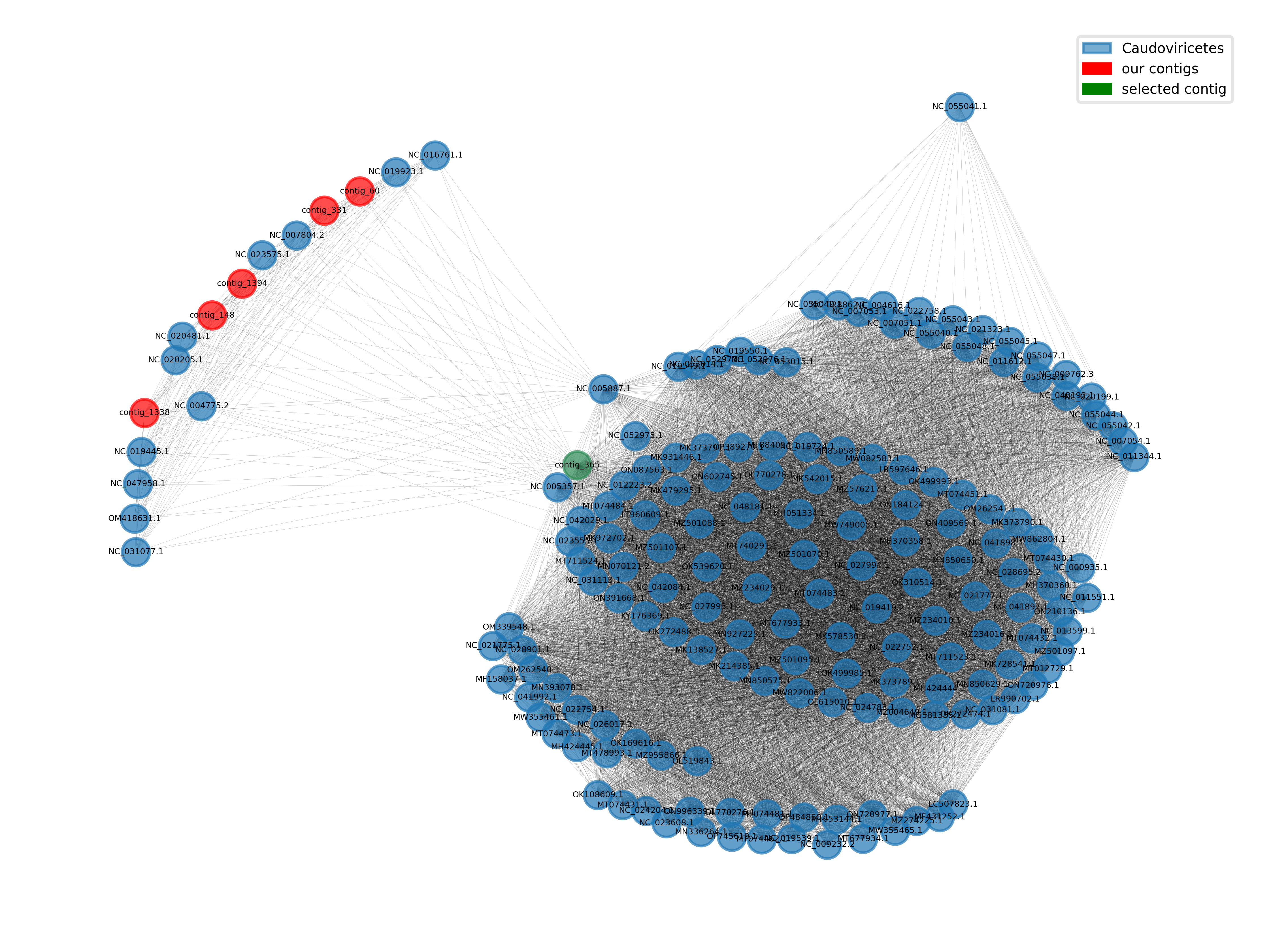
Today, you taxonomically annotated your phage contigs with vConTACT3.
The tool applies a gene-sharing network approach by computing the number of homologous genes between two viral sequences.
Based on this information, it integrates unseen contigs into a reference network of taxonomically classified phages, and then uses information about related viruses in the network to infer a taxonomic classification.
The resulting network, which contains both the reference phages and our assembled contigs, can be found in the output file graph.cyjs in your vConTACT3 results folder.
This file contains the network encoded in JSON format, which can be parsed with the Python standard library package json.
Python also provides several tools for handling and analyzing networks. In this section, you will use the NetworkX package to visualize the network of phages. The goal is to get an idea of the taxonomic diversity of the contigs in our dataset, and how it compares to reference phages in the database. You can either focus on a single contig and its closely related phages (close network neighborhood) or plot the whole network to get an overview of the full virosphere (at least the viruses in the reference database).
NetworkX provides several functions for drawing the network. Our network only consists of nodes (phages) and weighted edges (number of shared genes) between them, without any layout information (where to position the nodes). There are many algorithms for finding a visually pleasing layout for a given network. The Kamada-Kawai layout and the spring layout both employ a physical force-based simulation that optimizes the distance or attraction between node pairs. In our network, the number of shared genes between two nodes serves as a measure of attraction. The spring layout is computationally less demanding and should be used for the visualization of the complete network.
Making these plots involves a fair amount of programming and testing your code. This homework is not so much about figuring out the code but to introduce you to networkx as a tool for network analysis and visualization, and create a visualization which can confer the relational character of the data better than a table could. You can either try to figure out the code for this homework for yourself or start with one of the solutions and try to adjust or improve it. The goal is for you to end up with a picture of the network of phages which confers the idea of the algorithm VConTACT3 implements.
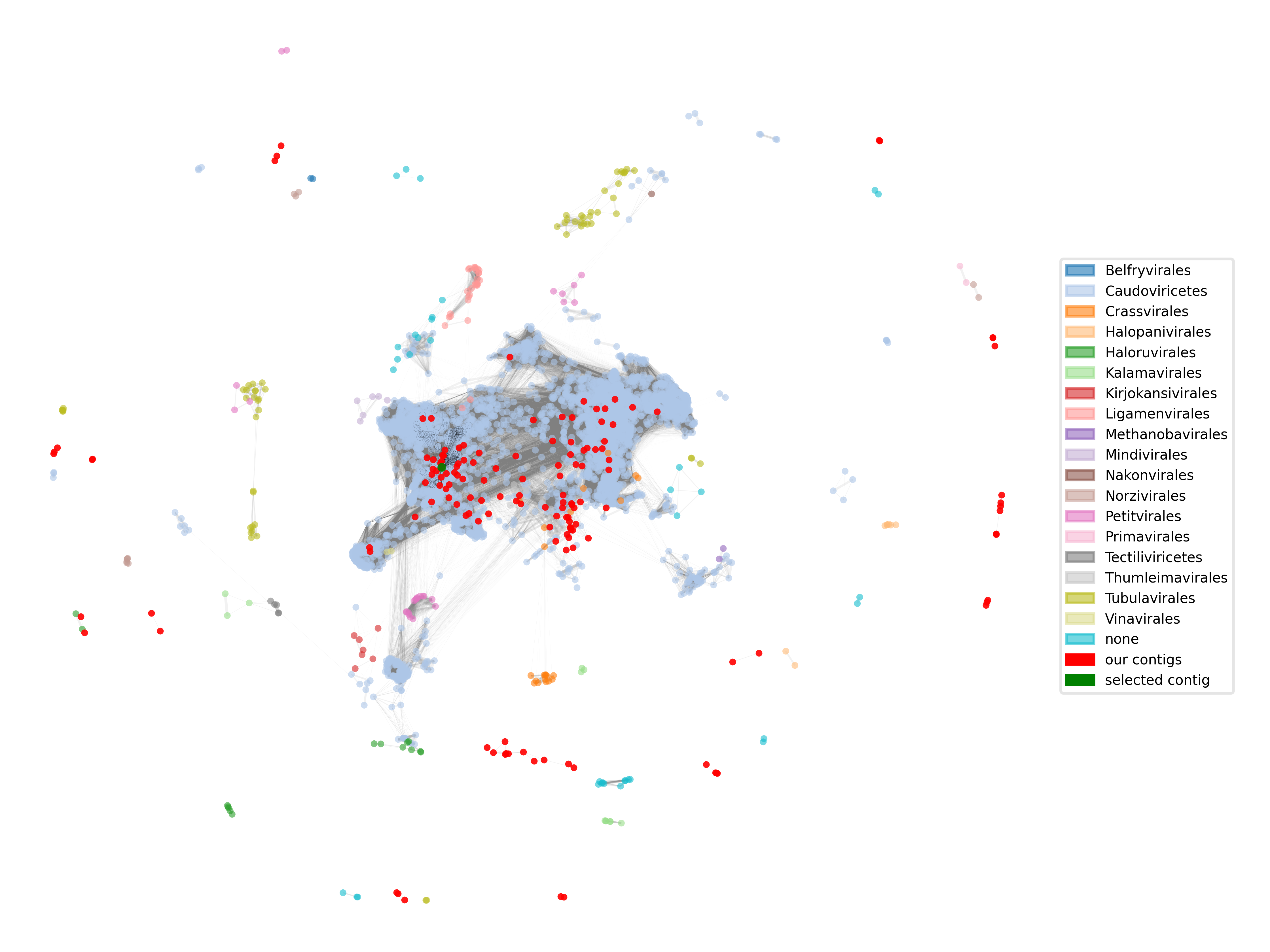
# you have to add networkx to the virtual environment first
import networkx as nx
# the json package is part of the standard library
import os, sys, json

# parse the json file and create a networkx graph from it
with open(graph_filename) as json_file:
     graph_json = json.load(json_file)

     # the following lines are necessary for compatibility with networkx
     graph_json["data"] = []
     graph_json["directed"] = False
     for node in graph_json["elements"]["nodes"]:
         # the 'value' attribute will be used for naming the nodes
         node["data"]["value"] = node["data"]["id"]

     # create a networkx graph from the graph_json dictionary
     g = nx.cytoscape_graph(graph_json)

# use draw_networkx_nodes(...) and draw_networkx_edges(...) to draw the graph
# use g.subgraph(...) or g.edge_subgraph(...) to select a subgraph of interest
python script for plotting the local neighborhood of your selected contig
import os, sys, json
import networkx as nx
import matplotlib.pyplot as plt
import matplotlib.patches as mpatches
import matplotlib as mpl

# the keys to access taxonomic ranks of the phages in the graph
ranks = ["order", "class", "phylum"]

# this function looks for the lowest available rank according to the ones defined in the ranks variable
def get_lowest_tax(node):
    for r in ranks:
        if r in node.keys(): return node[r]
    return "none"

def main():

    graph_filename = os.path.abspath(sys.argv[1])
    assert graph_filename.endswith(".cyjs")

    out_filename = os.path.abspath(sys.argv[2])
    assert out_filename.endswith(".png")

    contig_id = sys.argv[3]

    with open(graph_filename) as json_file:
        graph_json = json.load(json_file)

        # set for compatibility with networkx
        graph_json["data"] = []

        for node in graph_json["elements"]["nodes"]:
            # assign "value" attribute for compatibility
            node["data"]["value"] = node["data"]["id"]
            # assign lowest availble taxonomic rank with our function
            node["data"]["lowest_tax"] = get_lowest_tax(node["data"])

        g = nx.cytoscape_graph(graph_json)

    # find your favourite contig and get its internal node id
    contig_id_node = -1
    for node in g.nodes(data="name"):
    	if node[1] == contig_id: contig_id_node = node[0]

    # raise an error, if the contig could not be found
    if contig_id_node == -1: raise(AssertionError(f"Could not find {contig_id} in the graph"))

    # get all nodes connected to the selected contig and compute the corresponding subgraph
    node_set = {contig_id_node}.union({n for n in g.neighbors(contig_id_node)})
    subgraph =  g.subgraph(node_set)

    # get all taxa in the subgraph
    taxa = nx.get_node_attributes(subgraph, "lowest_tax")

    # set up a mapping from node to color based on the taxonomic rank
    unique_taxa = np.unique([t for t in taxa.values()])
    taxa_to_color = {t:mpl.colormaps["tab20"](i) for i, t in enumerate(unique_taxa)}
    colors = {n:taxa_to_color[t] for n, t in taxa.items()}

    # compute a positional layout using the kamada-kawai algorithm
    pos = nx.kamada_kawai_layout(subgraph)

    # set colors for nodes. use the taxonomic information to color the reference nodes
    names = nx.get_node_attributes(subgraph, "name")
    colors = [('seagreen' if names[n] == contig_id else 'red') if names[n].startswith('contig') else colors[n] for n in subgraph.nodes()]

    # draw the network using the functions networkx provides
    nx.draw_networkx_edges(subgraph, pos=pos, width=0.05, alpha=0.4)
    nx.draw_networkx_nodes(subgraph, pos=pos, alpha=0.7, node_size=100, node_color=colors)
    nx.draw_networkx_labels(subgraph, pos=pos, labels=names, font_size=3)

    # create rectangles for a legend connecting taxa with their colors in the graph
    patches = [mpatches.Patch(color=c, label=l, alpha=0.6) for l,c in taxa_to_color.items() if l!='none'] + \
   	   [mpatches.Patch(color='red', label='our contigs'), mpatches.Patch(color='green', label='selected contig')]

    plt.legend(handles=patches, loc='upper right', framealpha=0.5, frameon=True, prop={'size': 5})

    ax = plt.gca()
    ax.axis('off')
    plt.tight_layout()
    plt.savefig(out_filename, dpi=700)


if __name__ == "__main__":
    main()
python script for plotting the complete network of phages
import os, sys, json
import networkx as nx
import numpy as np
import matplotlib.pyplot as plt
import matplotlib.patches as mpatches
import matplotlib as mpl

# the keys to access taxonomic ranks of the phages in the graph
ranks = ["order", "class", "phylum"]

# this function looks for the lowest available rank according to the ones defined in the ranks variable
def get_lowest_tax(node):
    for r in ranks:
        if r in node.keys(): return node[r]
    return "none"

def main():

    # parse first parameter: path to the graph file
    graph_filename = os.path.abspath(sys.argv[1])
    assert graph_filename.endswith(".cyjs")

    # parse second parameter: path to the output file
    out_filename = os.path.abspath(sys.argv[2])
    assert out_filename.endswith(".png")

    # third parameter: the id of your favourite contig to highlight in the network
    contig_id = sys.argv[3]

	  # parse the json file containing the graph generated by VContact3
    with open(graph_filename) as json_file:
        graph_json = json.load(json_file)

        # set for compatibility with networkx
        graph_json["data"] = []

        for node in graph_json["elements"]["nodes"]:
            # assign "value" attribute for compatibility
            node["data"]["value"] = node["data"]["id"]
            # assign lowest availble taxonomic rank with our function
            node["data"]["lowest_tax"] = get_lowest_tax(node["data"])

        for edge in graph_json["elements"]["edges"]:
            # add "weight attribute for compatibility
            edge["data"]["weight"] = float(edge["data"]["distance"])
            # assign "attraction" attribute as inverse of "distance" for the position finding algorithm (spring)
            edge["data"]["attraction"] = 1-edge["data"]["weight"]

        # generate a networkx graph object from the json object
        g = nx.cytoscape_graph(graph_json)

    # find your favourite contig and get its internal node id
    contig_id_node = -1
    for node in g.nodes(data="name"):
    	if node[1] == contig_id: contig_id_node = node[0]

    # raise an error, if the contig could not be found
    if contig_id_node == -1: raise(AssertionError(f"Could not find {contig_id} in the graph"))

	  # limit our drawing to nodes actually connected to anything.
    connected_nodes = {n for n in g.nodes() if len(g.adj[n])>0}
    subgraph = g.subgraph(connected_nodes)

    # get all taxa in the subgraph
    taxa = nx.get_node_attributes(subgraph, "lowest_tax")

    # the number of taxa could be above the number of colors in a colormap, combine two for more colors
    colormap = [mpl.colormaps["tab20"](i) for i in range(20)] + [mpl.colormaps["tab20b"](i) for i in range(20)]

    # set up a mapping from node to color based on the taxonomic rank
    unique_taxa = np.unique([t for t in taxa.values()])
    taxa_to_color = {t:colormap[i] for i, t in enumerate(unique_taxa)}
    colors = {n:taxa_to_color[t] for n, t in taxa.items()}

    # compute positions for the nodes in the network. The spring algorithm is fast, but not so pretty.
    # sadly, networkx has no good alternatives for large networks.
    pos = nx.spring_layout(subgraph, k=1/100000, weight="attraction", iterations=50)

    # The produced layout is very concentrated in the center. Transform the coordinates for zooming in.
    pos = {k:np.array(p)-np.array(p)*np.log(np.linalg.norm(p)) for k,p in pos.items()}

    # get the "name" attribute of all nodes. We can use it to identify our contigs
    names = nx.get_node_attributes(subgraph, "name")

    # get the subgraph containing the reference set of phages and assign colors to the nodes according to the taxonomic rank
    nodes_ref = {n for n in subgraph.nodes() if not names[n].startswith("contig_")}
    subgraph_ref = subgraph.subgraph(nodes_ref)
    subgraph_ref_colors = [colors[n] for n in subgraph_ref.nodes()]

    # get the subgraph containing our contigs, we will color them all the same.
    nodes_contigs = {n for n in subgraph.nodes() if names[n].startswith("contig_")}
    subgraph_contigs = subgraph.subgraph(nodes_contigs)

    # get the subgraph of your favourite contig (only the contig :)) and the edge subgraph connecting the contig to the reference
    # we can use it to highlight the connections of the contig in the reference network
    subgraph_select = subgraph.subgraph({contig_id_node})
    subgraph_neighbors = subgraph.edge_subgraph([(contig_id_node, n) for n in subgraph.neighbors(contig_id_node)])

    # create a figure and axis with pyplot
    fig, ax = plt.subplots()

    # draw the reference network. first, we draw the edges and then the nodes. networkx also does this automatically.
    # read the comment of the next code block for setting the drawing order manually
    nx.draw_networkx_edges(subgraph, pos=pos, alpha=0.1, width=[1-subgraph[u][v]["weight"] for u,v in subgraph.edges()], node_size=10, edge_color="grey", ax=ax)
    nx.draw_networkx_nodes(subgraph_ref, pos=pos, alpha=0.6, node_size=10, node_color=subgraph_ref_colors, linewidths=0.0, ax=ax)

    # highlight your favourite contigs neighborhood by drawing the connecting edges and circles around the neighbor nodes
    # set_zorder tells matplotlib the order, in which objects are to be rendered. the values can be set arbitrarily as long as
    # they set up an order.
    edges_on_top = nx.draw_networkx_edges(subgraph_neighbors, pos=pos, alpha=0.6, width=0.02, node_size=10, ax=ax)
    edges_on_top.set_zorder(2)
    edges_on_top = nx.draw_networkx_nodes(subgraph_neighbors, pos=pos, linewidths=0.02, node_size=10, node_color='none', edgecolors="black", ax=ax)
    edges_on_top.set_zorder(2)

    # draw our contigs on top of everything else
    contig_nodes_collection = nx.draw_networkx_nodes(subgraph_contigs, pos=pos, alpha=0.9, node_size=10, node_color="red", linewidths=0.0, ax=ax)
    contig_nodes_collection.set_zorder(3)

    # add your favourite contig on top of that
    select_collection = nx.draw_networkx_nodes(subgraph_select, pos=pos, alpha=0.9, node_size=10, node_color="green", linewidths=0.0, ax=ax)
    select_collection.set_zorder(4)

    # create rectangles for a legend connecting taxa with their colors in the graph
    patches = [mpatches.Patch(color=c, label=l, alpha=0.6) for l,c in taxa_to_color.items()] + [mpatches.Patch(color='red', label='our contigs'), mpatches.Patch(color='green', label='selected contig')]
    ax.legend(handles=patches, loc='center right', framealpha=0.5, frameon=True, prop={'size': 5})

    # do some adjustments to improve the plot, first remove outer borders
    ax.axis('off')

    # set the min and max of each axis, add a bit of free space on the upper xlim for the legend
    xs, ys = [p[0] for p in pos.values()], [p[1] for p in pos.values()]
    xmin, xmax, ymin, ymax = np.min(xs), np.max(xs), np.min(ys), np.max(ys)
    ax.set_xlim([xmin + 0.05*xmin, xmax + 0.5*xmax])
    ax.set_ylim([ymin + 0.05*ymin, ymax + 0.05*ymax])

    # save the figure with a high resolution to be able to see enough
    fig.savefig(out_filename, dpi=700)


if __name__ == "__main__":
    main()
sbatch script for submitting the plotting script
#!/bin/bash
#SBATCH --tasks=1
#SBATCH --cpus-per-task=2
#SBATCH --partition=short
#SBATCH --mem=5G
#SBATCH --time=00:10:00
#SBATCH --job-name=taxonomic_graph
#SBATCH --output=./2.2_taxonomy/40_plot_networks/taxonomic_graph.slurm.%j.out
#SBATCH --error=./2.2_taxonomy/40_plot_networks/taxonomic_graph.slurm.%j.err

# activate the python virtual environment with the packages we need
source ../py3env/bin/activate

# in this sbatch script, its not necessarry to create the directory,
# we already told sbatch to create it for the log files.
mkdir -p ./2.2_taxonomy/40_plot_networks/

# define an array with contig ids to plot
declare -a arr=("contig_10" "contig_109", "contig_164")

# loop through the array
for contig in "${arr[@]}"
do
	# run our scripts for plotting the network around a contig of choice
  # PLOT CONTIG IN LOCAL GENE SHARING NETWORK
	python python_scripts/taxonomy/30_taxonomic_graph_local.py ../2.2_viral_taxonomy/02_vcontact3_results_new_contig_names/graph.cyjs ./2.2_taxonomy/40_plot_networks/"$contig"_graph_local.png $contig

  # PLOT CONTIG IN GLOBAL GENE SHARING NETWORK
  python python_scripts/taxonomy/30_taxonomic_graph_global.py ../2.2_viral_taxonomy/02_vcontact3_results_new_contig_names/graph.cyjs ./2.2_taxonomy/40_plot_networks/"$contig"_graph_global.png $contig
done


# deactivate the environment
deactivate
Plot the network of closely related phages
You can choose to plot the whole network of all reference phages and contigs, or zoom in and plot a single contig and its neighborhood.
- Use the taxonomic information encoded in the network to color the nodes.
- Use draw_networkx_nodes and draw_networkx_edges to better access the plot attributes.
Key Points
The Python package NetworkX can be used to work with networks
The visualization of graphs usually requires the computation of positions for the nodes
Many of our contigs are close to Caudoviricitae, but we also have several connected groups of unclassified sequences
Designing a research project
Overview
Teaching: min
Exercises: 480 minObjectives
Get acquainted with the state of the art of phage research
Choose one or more papers for inspiration
Write down 1 or 2 research questions
Make a plan on how to tackle the questions
To close off this course, we would like to give you the opportunity to design your own research project. A research question does not have to be very profound, it can be simple. Viromics is a new field, the virosphere is huge, and there is a LOT of data, so there are more unanswered than answered questions. Looking back on the course, are there things you are wondering about or want more time to work on? You can also look in literature for inspiration.
Here are a few papers that caught our eye, maybe they inspire you (feel free to find other papers too):
- A highly abundant bacteriophage discovered in the unknown sequences of human faecal metagenomes, by Dutilh et al (2014)
- Bacteriophage evolution differs by host, lifestyle and genome, by Mavrich and Hatfull (2017)
- Evolution of BACON Domain Tandem Repeats in crAssphage and Novel Gut Bacteriophage Lineages, by de Jonge et al (2019)
- Virus Bioinformatics, by Pappas et al (2021)
- High viral abundance and low diversity are associated with increased CRISPR-Cas prevalence across microbial ecosystems, by Meaden et al (2022)
- Viruses interact with hosts that span distantly related microbial domains in dense hydrothermal mats, by Hwang et al (2023)
Choose one type of project
Choose one type of project that better fits your interests:
- Go into detail into analyses
- Build a broader research proposal
Detailed Analyses
This type of project is more hands-on. You might write your own script(s), run your own analyses and produce your own plots. The idea here would be to focus on one of the methods/analyses we covered in the course and to go deeper into the analysis. In any case, the question you want to address should be clearly defined.
An example: “What are the differences between functional annotation done with Pharokka and Genomad?”.
Below are what should be included in your documentation/presentation for project type 1
- A brief background on the topic
- A workflow for the steps you plan to take
- A rationale for why you will take those steps
- What will be the inputs and outputs?
- Which programs will (do you plan to) use?
Note that hypotheses do not need be proven. We want to see from you as results:
Output (a table or a figure) Interpretation of the output: what does the data tell you? Does it answer your question? It does not have to. In a negative case, can you say what you might do differently next time
Research Proposal Style
This type of project is more in the style of a research proposal with a broader scope. You should focus on the biological questions and how to address them using viromics.
Your hypothesis and aims should be clear and backed-up by the literature.
Below are what should be included in your documentation/presentation for project type 2
- A brief background on the topic
- Formulate your research question or hypothesis to test
- What informed the question?
- How would you address this question or test the hypothesis? (make a detailed plan)
- Estimate the complexity of the problem
Presentation
- Present the project you worked on
- Limitations
- Things you found particularly interesting
- Any lessons learnt
Your project notes should still go into your lab book
Exercise
- Once you have an idea of a research question, take some time to talk about your idea with your fellow students. Often your initial idea can be further refined based on discussions with others.
- Make sure you check the literature: are there any papers that do something related to your question? Find the three papers that are the most closely related to your project, and use them to refine your question.
- Make a plan for tackling your question(s). The more detail you can add, the better. Think about data sources, bioinformatic methods, possible outcomes, expectations, backup/follow-up plans, hypotheses, and interpretation.
Here, you can find ideas for projects.
Key Points
Working on project
Overview
Teaching: min
Exercises: 180 minObjectives
Work on your own project
Clarify unclear points with your teachers
This morning please continue working on your research project design. Additionally, we have open hours with the teachers. Discuss the project and/or clarify any open issues with them.
Key Points
Prepare Presentation
Overview
Teaching: min
Exercises: 180 minObjectives
Prepare your final presentation
Take the time today to prepare your final presentation.
Key Points
Presentation
Overview
Teaching: min
Exercises: 180 minObjectives
Present your progress
Get feedback
Present your progress and get feedback from the teachers and your colleagues.
Key Points
Send Documentation
Overview
Teaching: min
Exercises: 180 minObjectives
Clean up documentation and scripts
Send all required documentation to your teachers
In your final hours on the module, clean up your lab book, scripts and any additional documentation and send them to your teachers. We hope you learned interesting things during the module and wish you all the best!
Key Points