Visualizing viral taxonomy

Overview

Teaching: 0 min
Exercises: 90 min

Objectives

Plot the network of closely related viruses created by vConTACT3

This section is suggested as homework.

Today, you taxonomically annotated your phage contigs with vConTACT3. The tool applies a gene-sharing network approach by computing the number of homologous genes between two viral sequences. Based on this information, it integrates unseen contigs into a reference network of taxonomically classified phages, and then uses information about related viruses in the network to infer a taxonomic classification. The resulting network, which contains both the reference phages and our assembled contigs, can be found in the output file graph.cyjs in your vConTACT3 results folder. This file contains the network encoded in JSON format, which can be parsed with the Python standard library package json.

Python also provides several tools for handling and analyzing networks. In this section, you will use the NetworkX package to visualize the network of phages. The goal is to get an idea of the taxonomic diversity of the contigs in our dataset, and how it compares to reference phages in the database. You can either focus on a single contig and its closely related phages (close network neighborhood) or plot the whole network to get an overview of the full virosphere (at least the viruses in the reference database).

NetworkX provides several functions for drawing the network. Our network only consists of nodes (phages) and weighted edges (number of shared genes) between them, without any layout information (where to position the nodes). There are many algorithms for finding a visually pleasing layout for a given network. The Kamada-Kawai layout and the spring layout both employ a physical force-based simulation that optimizes the distance or attraction between node pairs. In our network, the number of shared genes between two nodes serves as a measure of attraction. The spring layout is computationally less demanding and should be used for the visualization of the complete network.

Making these plots involves a fair amount of programming and testing your code. This homework is not so much about figuring out the code but to introduce you to networkx as a tool for network analysis and visualization, and create a visualization which can confer the relational character of the data better than a table could. You can either try to figure out the code for this homework for yourself or start with one of the solutions and try to adjust or improve it. The goal is for you to end up with a picture of the network of phages which confers the idea of the algorithm VConTACT3 implements.

# you have to add networkx to the virtual environment first
import networkx as nx
# the json package is part of the standard library
import os, sys, json

# parse the json file and create a networkx graph from it
with open(graph_filename) as json_file:
     graph_json = json.load(json_file)

     # the following lines are necessary for compatibility with networkx
     graph_json["data"] = []
     graph_json["directed"] = False
     for node in graph_json["elements"]["nodes"]:
         # the 'value' attribute will be used for naming the nodes
         node["data"]["value"] = node["data"]["id"]

     # create a networkx graph from the graph_json dictionary
     g = nx.cytoscape_graph(graph_json)

# use draw_networkx_nodes(...) and draw_networkx_edges(...) to draw the graph
# use g.subgraph(...) or g.edge_subgraph(...) to select a subgraph of interest

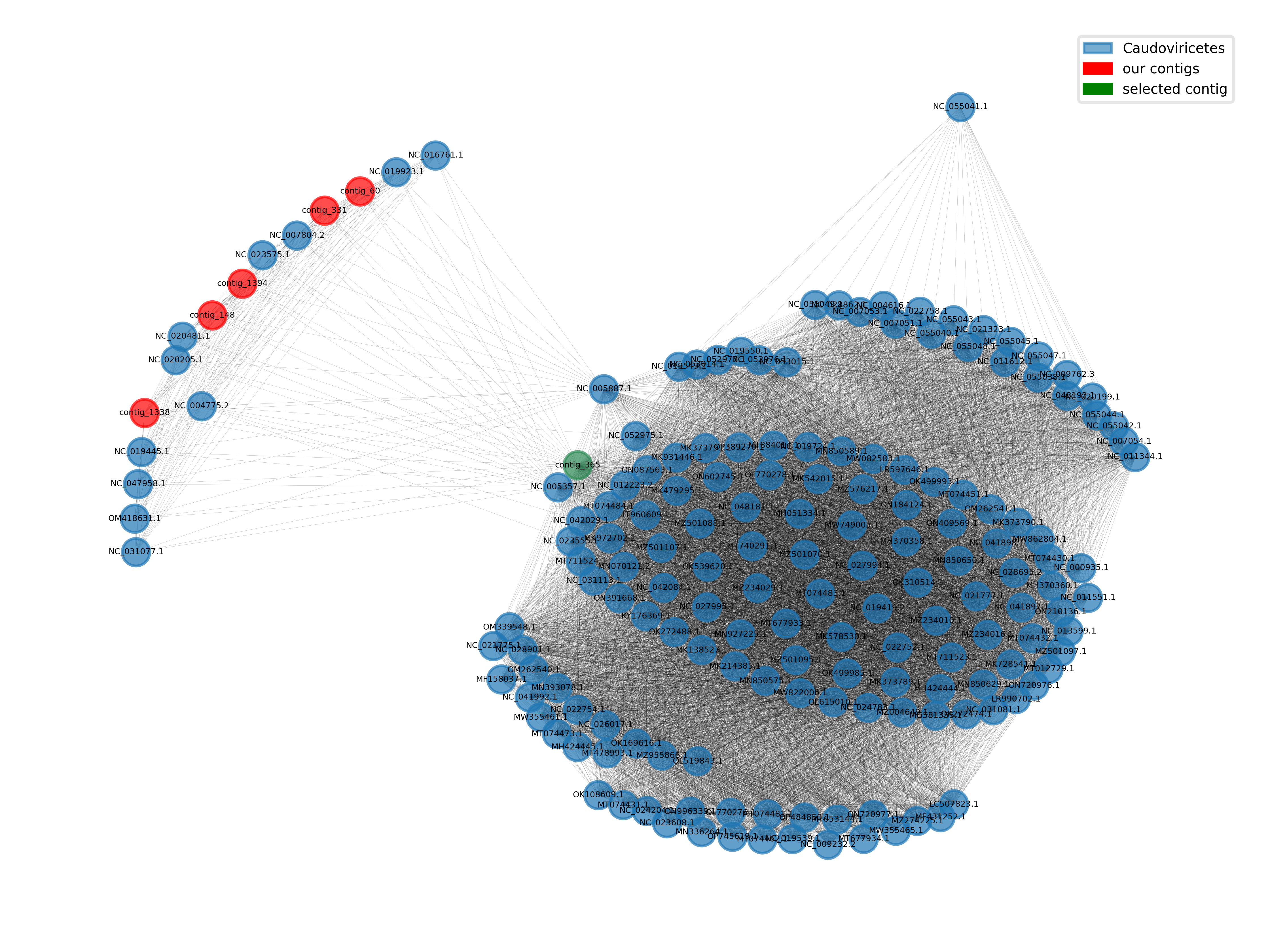
python script for plotting the local neighborhood of your selected contig

import os, sys, json
import networkx as nx
import matplotlib.pyplot as plt
import matplotlib.patches as mpatches
import matplotlib as mpl

# the keys to access taxonomic ranks of the phages in the graph
ranks = ["order", "class", "phylum"]

# this function looks for the lowest available rank according to the ones defined in the ranks variable
def get_lowest_tax(node):
    for r in ranks: 
        if r in node.keys(): return node[r]
    return "none"

def main():

    graph_filename = os.path.abspath(sys.argv[1])
    assert graph_filename.endswith(".cyjs")
    
    out_filename = os.path.abspath(sys.argv[2])
    assert out_filename.endswith(".png")

    contig_id = sys.argv[3]

    with open(graph_filename) as json_file:
        graph_json = json.load(json_file)

        # set for compatibility with networkx
        graph_json["data"] = []

        for node in graph_json["elements"]["nodes"]:
            # assign "value" attribute for compatibility
            node["data"]["value"] = node["data"]["id"]
            # assign lowest availble taxonomic rank with our function
            node["data"]["lowest_tax"] = get_lowest_tax(node["data"])

        g = nx.cytoscape_graph(graph_json)
        
    # find your favourite contig and get its internal node id
    contig_id_node = -1
    for node in g.nodes(data="name"):
    	if node[1] == contig_id: contig_id_node = node[0]
    
    # raise an error, if the contig could not be found
    if contig_id_node == -1: raise(AssertionError(f"Could not find {contig_id} in the graph"))

    # get all nodes connected to the selected contig and compute the corresponding subgraph
    node_set = {contig_id_node}.union({n for n in g.neighbors(contig_id_node)})
    subgraph =  g.subgraph(node_set)

    # get all taxa in the subgraph
    taxa = nx.get_node_attributes(subgraph, "lowest_tax")
    
    # set up a mapping from node to color based on the taxonomic rank
    unique_taxa = np.unique([t for t in taxa.values()])
    taxa_to_color = {t:mpl.colormaps["tab20"](i) for i, t in enumerate(unique_taxa)}
    colors = {n:taxa_to_color[t] for n, t in taxa.items()}

    # compute a positional layout using the kamada-kawai algorithm
    pos = nx.kamada_kawai_layout(subgraph)

    # set colors for nodes. use the taxonomic information to color the reference nodes
    names = nx.get_node_attributes(subgraph, "name")
    colors = [('seagreen' if names[n] == contig_id else 'red') if names[n].startswith('contig') else colors[n] for n in subgraph.nodes()]

    # draw the network using the functions networkx provides
    nx.draw_networkx_edges(subgraph, pos=pos, width=0.05, alpha=0.4)
    nx.draw_networkx_nodes(subgraph, pos=pos, alpha=0.7, node_size=100, node_color=colors)
    nx.draw_networkx_labels(subgraph, pos=pos, labels=names, font_size=3)

    # create rectangles for a legend connecting taxa with their colors in the graph
    patches = [mpatches.Patch(color=c, label=l, alpha=0.6) for l,c in taxa_to_color.items() if l!='none'] + \
   	   [mpatches.Patch(color='red', label='our contigs'), mpatches.Patch(color='green', label='selected contig')]
   	
    plt.legend(handles=patches, loc='upper right', framealpha=0.5, frameon=True, prop={'size': 5})

    ax = plt.gca()
    ax.axis('off')
    plt.tight_layout()
    plt.savefig(out_filename, dpi=700)


if __name__ == "__main__":
    main()

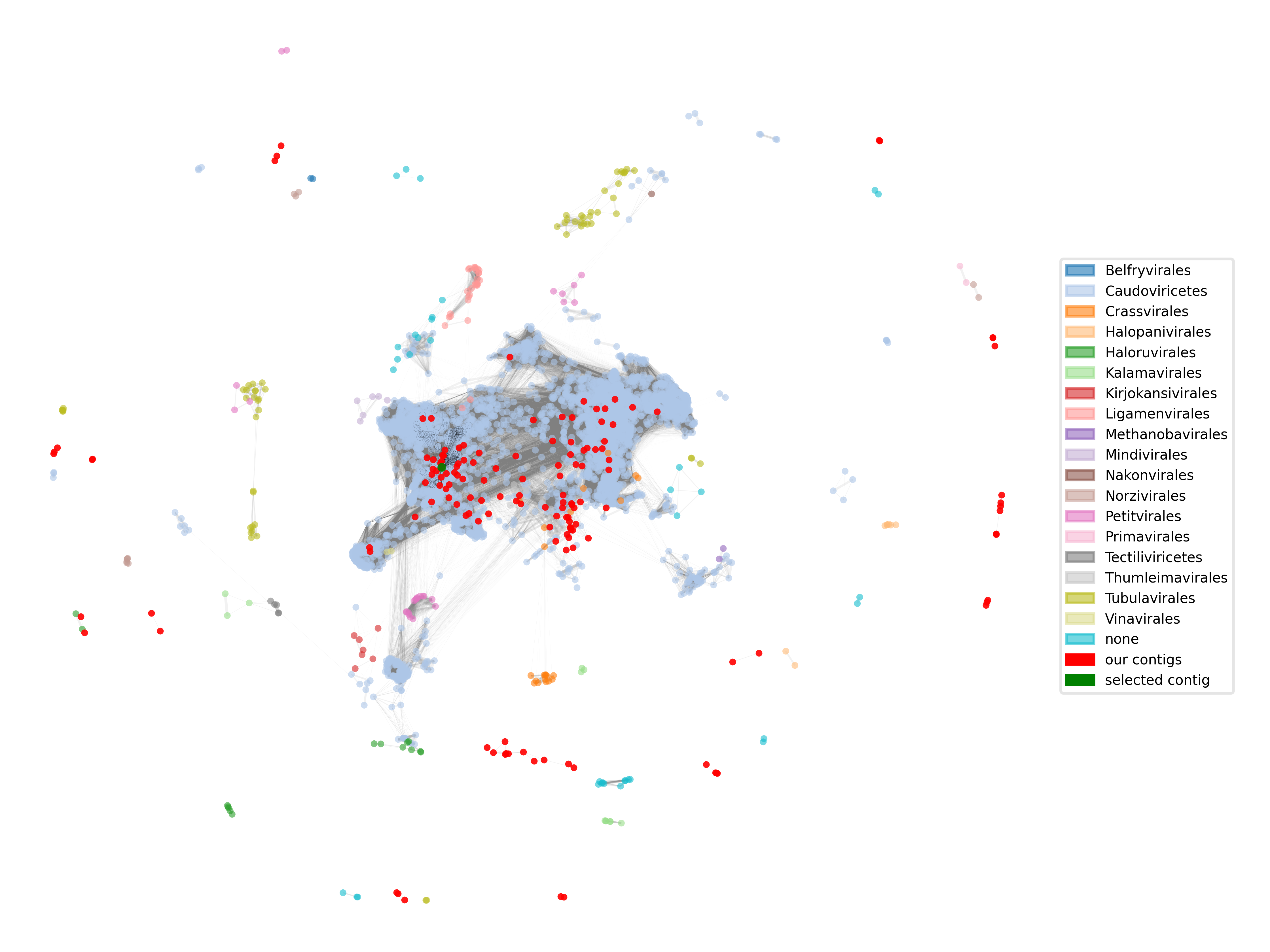
python script for plotting the complete network of phages

import os, sys, json
import networkx as nx
import numpy as np
import matplotlib.pyplot as plt
import matplotlib.patches as mpatches
import matplotlib as mpl

# the keys to access taxonomic ranks of the phages in the graph
ranks = ["order", "class", "phylum"]

# this function looks for the lowest available rank according to the ones defined in the ranks variable
def get_lowest_tax(node):
    for r in ranks: 
        if r in node.keys(): return node[r]
    return "none"

def main():

    # parse first parameter: path to the graph file
    graph_filename = os.path.abspath(sys.argv[1])
    assert graph_filename.endswith(".cyjs")
    
    # parse second parameter: path to the output file
    out_filename = os.path.abspath(sys.argv[2])
    assert out_filename.endswith(".png")

    # third parameter: the id of your favourite contig to highlight in the network
    contig_id = sys.argv[3]

	  # parse the json file containing the graph generated by VContact3
    with open(graph_filename) as json_file:
        graph_json = json.load(json_file)
   
        # set for compatibility with networkx
        graph_json["data"] = []
        
        for node in graph_json["elements"]["nodes"]:
            # assign "value" attribute for compatibility
            node["data"]["value"] = node["data"]["id"]
            # assign lowest availble taxonomic rank with our function
            node["data"]["lowest_tax"] = get_lowest_tax(node["data"])
            
        for edge in graph_json["elements"]["edges"]:
            # add "weight attribute for compatibility
            edge["data"]["weight"] = float(edge["data"]["distance"])
            # assign "attraction" attribute as inverse of "distance" for the position finding algorithm (spring)
            edge["data"]["attraction"] = 1-edge["data"]["weight"]
            
        # generate a networkx graph object from the json object    
        g = nx.cytoscape_graph(graph_json)
    
    # find your favourite contig and get its internal node id
    contig_id_node = -1
    for node in g.nodes(data="name"):
    	if node[1] == contig_id: contig_id_node = node[0]
    
    # raise an error, if the contig could not be found
    if contig_id_node == -1: raise(AssertionError(f"Could not find {contig_id} in the graph"))

	  # limit our drawing to nodes actually connected to anything.
    connected_nodes = {n for n in g.nodes() if len(g.adj[n])>0}
    subgraph = g.subgraph(connected_nodes)
    
    # get all taxa in the subgraph
    taxa = nx.get_node_attributes(subgraph, "lowest_tax")
    
    # the number of taxa could be above the number of colors in a colormap, combine two for more colors
    colormap = [mpl.colormaps["tab20"](i) for i in range(20)] + [mpl.colormaps["tab20b"](i) for i in range(20)]
    
    # set up a mapping from node to color based on the taxonomic rank
    unique_taxa = np.unique([t for t in taxa.values()])
    taxa_to_color = {t:colormap[i] for i, t in enumerate(unique_taxa)}
    colors = {n:taxa_to_color[t] for n, t in taxa.items()}

    # compute positions for the nodes in the network. The spring algorithm is fast, but not so pretty.
    # sadly, networkx has no good alternatives for large networks.
    pos = nx.spring_layout(subgraph, k=1/100000, weight="attraction", iterations=50)
    
    # The produced layout is very concentrated in the center. Transform the coordinates for zooming in.
    pos = {k:np.array(p)-np.array(p)*np.log(np.linalg.norm(p)) for k,p in pos.items()}
    
    # get the "name" attribute of all nodes. We can use it to identify our contigs
    names = nx.get_node_attributes(subgraph, "name")
    
    # get the subgraph containing the reference set of phages and assign colors to the nodes according to the taxonomic rank
    nodes_ref = {n for n in subgraph.nodes() if not names[n].startswith("contig_")}
    subgraph_ref = subgraph.subgraph(nodes_ref)
    subgraph_ref_colors = [colors[n] for n in subgraph_ref.nodes()]
    
    # get the subgraph containing our contigs, we will color them all the same.
    nodes_contigs = {n for n in subgraph.nodes() if names[n].startswith("contig_")}
    subgraph_contigs = subgraph.subgraph(nodes_contigs)
    
    # get the subgraph of your favourite contig (only the contig :)) and the edge subgraph connecting the contig to the reference
    # we can use it to highlight the connections of the contig in the reference network
    subgraph_select = subgraph.subgraph({contig_id_node})
    subgraph_neighbors = subgraph.edge_subgraph([(contig_id_node, n) for n in subgraph.neighbors(contig_id_node)])

    # create a figure and axis with pyplot
    fig, ax = plt.subplots()

    # draw the reference network. first, we draw the edges and then the nodes. networkx also does this automatically. 
    # read the comment of the next code block for setting the drawing order manually
    nx.draw_networkx_edges(subgraph, pos=pos, alpha=0.1, width=[1-subgraph[u][v]["weight"] for u,v in subgraph.edges()], node_size=10, edge_color="grey", ax=ax)
    nx.draw_networkx_nodes(subgraph_ref, pos=pos, alpha=0.6, node_size=10, node_color=subgraph_ref_colors, linewidths=0.0, ax=ax)
    
    # highlight your favourite contigs neighborhood by drawing the connecting edges and circles around the neighbor nodes
    # set_zorder tells matplotlib the order, in which objects are to be rendered. the values can be set arbitrarily as long as
    # they set up an order.
    edges_on_top = nx.draw_networkx_edges(subgraph_neighbors, pos=pos, alpha=0.6, width=0.02, node_size=10, ax=ax)
    edges_on_top.set_zorder(2)
    edges_on_top = nx.draw_networkx_nodes(subgraph_neighbors, pos=pos, linewidths=0.02, node_size=10, node_color='none', edgecolors="black", ax=ax)
    edges_on_top.set_zorder(2)
    
    # draw our contigs on top of everything else
    contig_nodes_collection = nx.draw_networkx_nodes(subgraph_contigs, pos=pos, alpha=0.9, node_size=10, node_color="red", linewidths=0.0, ax=ax)
    contig_nodes_collection.set_zorder(3)
    
    # add your favourite contig on top of that
    select_collection = nx.draw_networkx_nodes(subgraph_select, pos=pos, alpha=0.9, node_size=10, node_color="green", linewidths=0.0, ax=ax)
    select_collection.set_zorder(4)
    
    # create rectangles for a legend connecting taxa with their colors in the graph
    patches = [mpatches.Patch(color=c, label=l, alpha=0.6) for l,c in taxa_to_color.items()] + [mpatches.Patch(color='red', label='our contigs'), mpatches.Patch(color='green', label='selected contig')]
    ax.legend(handles=patches, loc='center right', framealpha=0.5, frameon=True, prop={'size': 5})
    
    # do some adjustments to improve the plot, first remove outer borders
    ax.axis('off')
    
    # set the min and max of each axis, add a bit of free space on the upper xlim for the legend
    xs, ys = [p[0] for p in pos.values()], [p[1] for p in pos.values()]
    xmin, xmax, ymin, ymax = np.min(xs), np.max(xs), np.min(ys), np.max(ys)
    ax.set_xlim([xmin + 0.05*xmin, xmax + 0.5*xmax])
    ax.set_ylim([ymin + 0.05*ymin, ymax + 0.05*ymax])
    
    # save the figure with a high resolution to be able to see enough
    fig.savefig(out_filename, dpi=700)


if __name__ == "__main__":
    main()

sbatch script for submitting the plotting script

#!/bin/bash
#SBATCH --tasks=1
#SBATCH --cpus-per-task=2
#SBATCH --partition=short
#SBATCH --mem=5G
#SBATCH --time=00:10:00
#SBATCH --job-name=taxonomic_graph
#SBATCH --output=./2.2_taxonomy/40_plot_networks/taxonomic_graph.slurm.%j.out
#SBATCH --error=./2.2_taxonomy/40_plot_networks/taxonomic_graph.slurm.%j.err

# activate the python virtual environment with the packages we need
source ../py3env/bin/activate

# in this sbatch script, its not necessarry to create the directory,
# we already told sbatch to create it for the log files.
mkdir -p ./2.2_taxonomy/40_plot_networks/

# define an array with contig ids to plot
declare -a arr=("contig_10" "contig_109", "contig_164")

# loop through the array
for contig in "${arr[@]}"
do
	# run our scripts for plotting the network around a contig of choice
  # PLOT CONTIG IN LOCAL GENE SHARING NETWORK
	python python_scripts/taxonomy/30_taxonomic_graph_local.py ../2.2_viral_taxonomy/02_vcontact3_results_new_contig_names/graph.cyjs ./2.2_taxonomy/40_plot_networks/"$contig"_graph_local.png $contig

  # PLOT CONTIG IN GLOBAL GENE SHARING NETWORK
  python python_scripts/taxonomy/30_taxonomic_graph_global.py ../2.2_viral_taxonomy/02_vcontact3_results_new_contig_names/graph.cyjs ./2.2_taxonomy/40_plot_networks/"$contig"_graph_global.png $contig
done


# deactivate the environment
deactivate

Plot the network of closely related phages

You can choose to plot the whole network of all reference phages and contigs, or zoom in and plot a single contig and its neighborhood.

Use the taxonomic information encoded in the network to color the nodes.

Use draw_networkx_nodes and draw_networkx_edges to better access the plot attributes.

Key Points

The Python package NetworkX can be used to work with networks

The visualization of graphs usually requires the computation of positions for the nodes

Many of our contigs are close to Caudoviricitae, but we also have several connected groups of unclassified sequences

previous episode

Viromics2024

next episode